Alan Hodgkin and Andrew Huxley received the Nobel prize in 1963 for their creation of a mathematical model that accurately explained the propagation of action potentials in the squid giant axon. Versions of this model can quantify action potential generation and propagation in all neurons, including yours.
The Model
Let's implement the Hodgkin-Huxley model to simulate an action potential. Let's begin by considering a single neuron. Or rather, the axon of a neuron. This (simplified) axon contains two ion channels, the voltage-gated Na+ channel and the voltage-gated K+ channel. This axon we are constructing also has the nice property that its voltage is uniform throughout, and is directly proportional to the charge stored on the inside of its membrane. In other words, our axon is a capacitor. The equation for a capacitor is
\begin{equation} C = Q/V \end{equation}
where C is capacitance, V is voltage, and Q is the charge stored in the membrane. You can see that as the charge stored in the membrane doubles, the voltage also doubles. We can rearrange this equation to look like this:
\begin{equation} CV=Q \end{equation}
If we differentiate with respect to time, we get this:
\begin{equation} C \frac{dV}{dt} = I \end{equation}
where I is current, since current is simply the rate of change of charge over time. This equation is also known as the 'single-compartment model'. It is the basis of our model. This equation indicates that we can know the rate of change of the voltage if we know the current passing through the ion channels in our axon. If the capacitance is 1nF (capacitance won't change over time, so it is a constant in our model) and the current I=10 nA, then rate of change of voltage is 10 V/s. If our starting voltage was -50mV, then over 1 ms our voltage would increase by 10mV, and at the end of that millisecond would be at -40 mV.
Where do Hodgkin and Huxley come into this? We only have two classes of ion channels (Na+ and K+), so the current flowing into our axon should be the sum of the currents flowing through these ion channels. Once we know the currents, we can get the voltage, which is ultimately what we are interested in. This is where Hodgkin and Huxley help us.
The delayed-rectifier K+ channel
According to Ohm's law, when the voltage (relative to equilibrium potential \(E\)) across a membrane doubles, current across the membrane doubles. Another (stronger) way of saying that is that voltage and current are linearly related:
\begin{equation} ( V - E ) g = I \end{equation}
\(E\) is the equilibrium potential for that channel. \(g\) stands for conductance, the constant of proportionality. You can think of the conductance as how easy it is for charged ions to get across the membrane. Conductance goes up when the number of channels open goes up. This relationship is also linear: if 5 ion channels are open, the total conductance through the membrane is 5 times greater than if a single channel was open. The total conductance for a single class of ion channels at any given time equals the maximum possible conductance for those ion channels times the probability that each one is open. If the total conductance for all K+ was 100 nS, and the probability of any given channel being open is .5, then the conductance would be 50 nS. We started out wanting to know what the current flowing through the K+ channels is. Now the problem reduces to, what is the open probability of a channel at a given time?
Without going through the experimental details, Hodgkin and Huxley figured that out for us. The delayed-rectifier K+ channel is composed of four subunits, each one of which must undergo a conformational change if the channel is going to open. Let's let \(n\) be the probability that a single subunit is in its open position. Then the probability that all four subunits are in the open position is \(n^4\). In equation form:
\begin{equation} P(K^{+}_{open}) = n^{4} \end{equation}
Now lets focus on that variable \(n\) . The subunit is going back and forth between being in its open and closed conformation. Like any chemical reaction, the rate going from one state to another will be proportional to the starting state. The rate going from the open state to the closed state will be porportional to \(n\), and the rate going from the closed state to the open state will be proportional to \(1-n\). Also, there is a voltage dependence for both the open and closing rates. Let's call the voltage dependence of the opening rate \(\alpha_n(V)\) and the closing rate \(\beta_n(V)\). Putting all this together, the overall rate of transition will be the sum of the forward and backward parts:
We will use this equation to model how all the subunits open and close. For the delayed-rectifier K+ channel, Hodgkin and Huxley found equations for the voltage dependencies:
The voltage gated Na+ channel
Things only get slightly more complicated for the Na+ channel, but all the logic we used with the K+ channel applies. We can model the Na+ channel with four subunits also, and all of them must be open for the channel to be open. The difference is, one of those subunits will have a different voltage dependency, so we need to treat it separately. Let's use \(m\) to represent the probability that a normal subunit is open. By 'normal', I mean that as the voltage increases, this subunit is more likely to be in its open conformation. Let's use \(h\) to represent the probability that the oddball subunit is open. These two subunit types have opening and closing voltage dependent rates which Hodgkin and Huxley found, so let's write those out:
Similar to the K+ channel, the probability that the channel is open is the product of the probabilities that all the subunits are in their open conformational state:
Putting it all together
As I stated earlier, the total current through the membrane is the sum of all the individual components. We've mentioned two kinds of ion channels, but let's add one more to make our model complete. An axon at rest has some ion channels open. These are permeable mostly to K+. There is more K+ inside most mammalian cells than outside of them, so if a K+ permeable channel opens, they will diffuse down their concentration gradient and out of the cell. This makes the cell more negative. This is why at rest, most cells have a negative voltage. The resting conductance (mostly K+) is called the leak conductance, \(g_L\). Now we can write an equation for the total current through the cell.
Now we have all the equations we need to construct our model. In our model, we will have a starting voltage. We will use that voltage to figure out what state all our channels are in, and use that to get the current. When we have the current, we can get the change in voltage, and add that \(\Delta V\) to the voltage from our previous step.
In more detail, the algorithm goes like this:
- Initialize a starting voltage, and states for all the subunits.
- Using that starting voltage, determine what the opening and closing rates of all the subunits is (All those \(\alpha\)s and \(\beta\)s).
- Use those subunits' rates to determine the open probability of each ion channel.
- Use the open probabilities to determine the currents flowing through them into the cell.
- Sum up these currents and calculate how much the voltage will change
We will perform all those steps for every time step, using the voltage from the previous time step to calculate the voltage for the next. It sounds like a lot of work, but in our model, most of that work will be performed on the computer for you!! You just have to input the equations! Sound easy? Let's start.
Step 1
Write a function for total current equation $$I=g_L(V-E_L)+g_K n^4(V-E_K) + g_{Na} m^3h(V-E_{Na}) $$
import numpy as np
import matplotlib.pyplot as plt
from __future__ import division
%matplotlib inline

g_L=.003 #mS/mm^2
g_K=.36  #mS/mm^2
g_Na=1.2 #mS/mm^2
E_L=-54.387  #mV
E_K=-77 #mV
E_Na=50 #mV
def getCurrent(V, n, m, h):
    I=  g_L*(V-E_L)  +  g_K*(n**4)*(V-E_K)   +   g_Na*(m**3)*h*(V-E_Na)
    return -I
Step 2
Write functions for all the \(\alpha(V)\) and \(\beta(V)\) equations.
def alpha_n(V):
    return (.01*(V+55))/(1-np.exp(-.1*(V+55))) #from Dayan & Abbott
def beta_n(V):
    return 0.125*np.exp(-0.0125*(V+65)) #from Dayan & Abbott
def alpha_m(V):
    return (.1*(V+40))/(1-np.exp(-.1*(V+40))) #from Dayan & Abbott
def beta_m(V):
    return 4*np.exp(-.0556*(V+65)) #from Dayan & Abbott
def alpha_h(V):
    return .07*np.exp(-.05*(V+65)) #from Dayan & Abbott
def beta_h(V):
    return 1./(1.+np.exp(-.1*(V+35))) #from Dayan & Abbott
Step 3
Write a function for the rate of change of the state of each subunit. This function should take as inputs 1) the type of subunit, 2) the voltage, and 3) the current state. It should output the rate the subunit is changing. It should also call the functions written in step 2.
def getSubunitChangeRate(subunit_type,V,currState):
    if subunit_type=='n':
        alpha=alpha_n(V)
        beta=beta_n(V)
    elif subunit_type=='m':
        alpha=alpha_m(V)
        beta=beta_m(V)
    elif subunit_type=='h':
        alpha=alpha_h(V)
        beta=beta_h(V)
    return alpha*(1-currState)-beta*currState
Step 4
Write a function that will get the voltage at the next step given the current voltage
set \(C=.01\) nF/cm2
def updateVoltage(V_old,n,m,h,dt,external_current=0):
    C= .01 #nF/cm^2
    # for each subunit type, update the probability that subunit is in its 'open' conformation
    n=n+dt*getSubunitChangeRate('n',V_old,n)
    m=m+dt*getSubunitChangeRate('m',V_old,m)
    h=h+dt*getSubunitChangeRate('h',V_old,h)
    I=getCurrent(V_old,n,m,h)+external_current
    V_new=V_old+dt*(I/C)
    return V_new, n, m, h
Step 5
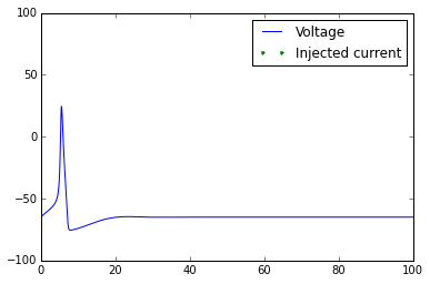
Plot an action potential
dt=.025
simTime=100
t=np.arange(0,simTime,dt)
V=np.zeros(len(t))
n=np.zeros(len(t))
m=np.zeros(len(t))
h=np.zeros(len(t))
external_current=np.zeros(len(t))
V[0]=-65
n[0]=0#alpha_n(V[0])/(alpha_n(V[0])+beta_n(V[0])) #this is the value at this voltage at t=infinity
m[0]=0#alpha_m(V[0])/(alpha_m(V[0])+beta_m(V[0])) #this is the value at this voltage at t=infinity
h[0]=0#alpha_h(V[0])/(alpha_h(V[0])+beta_h(V[0])) #this is the value at this voltage at t=infinity

#external_current[(t>5)*(t<6)]=.2
#external_current[(t>30)*(t<31)]=.2
#external_current[(t>50)*(t<80)]=.2

for i in range(1,len(V)):
    V[i],n[i],m[i],h[i]=updateVoltage(V[i-1],n[i-1],m[i-1],h[i-1],dt,external_current[i-1])
plt.plot(t,V)
t_current=t[external_current>0]
plt.plot(t_current,-90*np.ones(len(t_current)),linestyle='None',marker='.')
plt.axis([0,np.max(t),-100,100])
plt.legend(['Voltage','Injected current'])
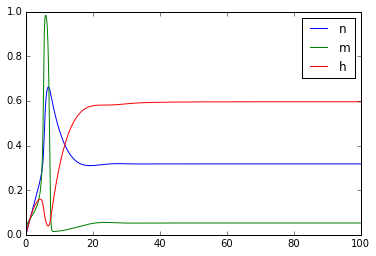
plt.figure()
plt.plot(t,n)
plt.plot(t,m)
plt.plot(t,h)
plt.legend(['n','m','h'])
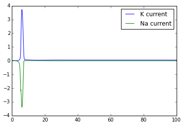
plt.figure()
plt.plot(t,g_K*(n**4)*(V-E_K) )
plt.plot(t,g_Na*(m**3)*h*(V-E_Na))
plt.legend(['K current','Na current'])
Once you've got this working, try playing with the external_current to generate multiple action potentials.
Congratulations! You've implemented the Hodgkin-Huxley model!