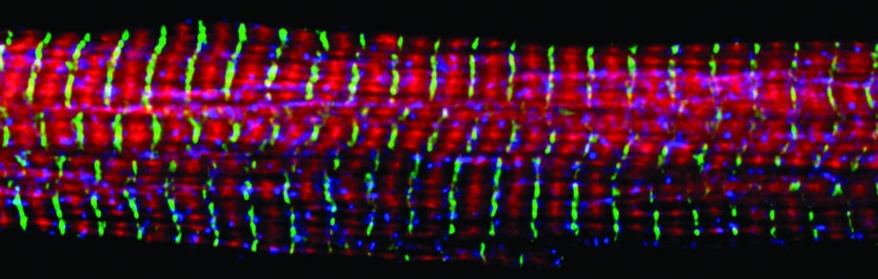
In this post, I'll describe an algorithm I developed for detection of muscle fibers that have been stained with a fluorescently conjugated anti-laminin antibody. While this project was motivated by learning how muscles regenerate after damage, detection of individual fibers is the first step in many possible analyses of muscles.
Set up
We'll be using the Python programming language and flika, an image analysis program. To download and install flika, run:
pip install flika
We'll also be using the python packages numpy, scipy, scikit-image and scikit-learn. Let's import flika, the other packages, and open our image.
import numpy as np
import scipy
import skimage
from sklearn import svm
from flika import *
start_flika()
# This displays the image in an interactive window
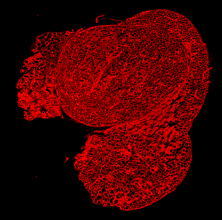
muscle_window = open_file('path/to/muscle_file.tif')
I = muscle_window.image
Thresholding with borders
One apparent method for fiber detection is to simply threshold the image at some value midway between black level and saturation and look for contiguous regions of pixels. However, if the threshold is set high, many gaps appear between fibers and multiple fibers will be counted as a single fiber. If the threshold is set low, the measured size of the cell bodies will shrink. How can we solve the problem?
Let's start with a low threshold in order to detect contiguous pixels that we are sure are located within a single myocyte. We can use scikit-image's label function to find all the contiguous regions of pixels. Then we can threshold using a slightly higher threshold.
from skimage.measure import label
thresh1 = .2
thresh2 = .3
label_im_1 = label(I < thresh1, connectivity=2)
label_im_2 = label(I < thresh2, connectivity=2)
Because we are using a higher threshold for label_im_2, cells that ought to be considered separate will merge together. We can check for this by comparing the labels with different thresholds and looking for large perimeter increases. If we see a large perimeter increase, we can be confident that one label merged with another.
from skimage import measure
props_1 = measure.regionprops(label_im_1)
props_2 = measure.regionprops(label_im_2)
roi_num = 1
prop1 = props_1[roi_num]
x, y = prop1.coords[0,:]
prop2 = props_2[label_im_2[x, y] - 1]
perim_ratio = prop2.perimeter/prop1.perimeter
print(perim_ratio)

2.06654889942
In this example, the perimeter of our ROI (region of interest) more than doubled. This strongly suggests that our fiber merged with another one. To prevent this merge, we can build a border between the two cells at their boundary. Here is a function to get the boundary between two ROIs:
from skimage.morphology import binary_dilation

def get_border_between_two_props(prop1, prop2):
    I2 = np.copy(prop2.image)
    I1 = np.zeros_like(I2)
    bbox = np.array(prop2.bbox)
    top_left = bbox[:2]
    a = prop1.coords - top_left
    I1[a[:, 0], a[:, 1]] = 1
    I1_expanded1 = binary_dilation(I1)
    I1_expanded2 = binary_dilation(binary_dilation(I1_expanded1))
    I1_expanded2[I1_expanded1] = 0
    border = I1_expanded2 * I2
    return np.argwhere(border) + top_left
Now that we have this function, we can check if the perimeter increase exceeds a threshold. If it does, we will add the border between the two ROIs to the original image.
borders = np.zeros_like(I)
if perim_ratio > 1.5:
    border_idx = get_border_between_two_props(prop1, prop2)
    borders[border_idx[:,0], border_idx[:, 1]] = 1
I[np.where(borders)] = 2
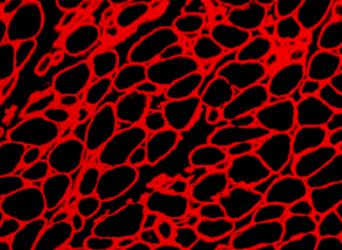
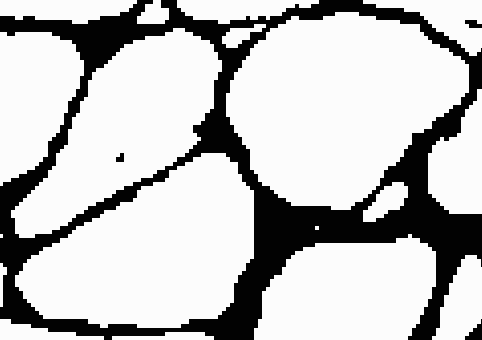
After adding the border, if we threshold using the high threshold, both cells will remain distinct. To complete this process, we can iterate through this procedure using different pairs of thresholds each time. We start with two low thresholds, look for sets of cells that merge between the thresholds, add borders between them, increase the thresholds, and repeat the process. Then we can safely threshold at the highest threshold without risk of merging. The result looks like this.
Classification of fibers
Each region in the original image is either fiber or space between fibers. Now that we have separated fibers from each other, we need to classify each contiguous ROI as a fiber or not. To do that, we can use a support vector machine. First, we need to identify features that might distinguish fibers from not. After trial and error, I settled on area, eccentricity, convexity, and circularity.
label_im = I > .8
props = measure.regionprops(label_im)
area = np.array([p.filled_area for p in props])
eccentricity = np.array([p.eccentricity for p in props])
convexity = np.array([p.filled_area / p.convex_area for p in props])
perimeter = np.array([p.perimeter for p in props])
circularity = np.empty_like(perimeter)
for i in np.arange(len(circularity)):
    if perimeter[i] == 0:
        circularity[i] = 0
    else:
        circularity[i] = (4 * np.pi * area[i]) / perimeter[i]**2
features_array = np.array([area, eccentricity, convexity, circularity]).T
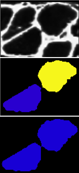
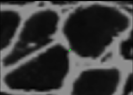
Now that we have our features, we need to label a subset of them as positives and negatives. I wrote a GUI which allows a user to click an ROI to label it as a positive (green) or a negative (red). I won't display the code here, but you can find it in the myoquant plugin.
Once you have labeled several positive and negative ROIs, we can use those ROIs as the training set. Before we train our SVM on them, we need to normalize the data.
def get_norm_coeffs(X):
    mean = np.mean(X, 0)
    std = np.std(X, 0)
    return mean, std

def normalize_data(X, mean, std):
    X = X - mean
    X = X / (2 * std)
    return X

X_train, y = get_training_data()
mu, sigma = get_norm_coeffs(X_train)
X_train_norm = normalize_data(X_train, mu, sigma)
Now we can train the SVM, and classify our unlabeled data.
X_test = normalize_data(get_testing_data(), mu, sigma)
clf = svm.SVC(kernel='linear')
clf.fit(X_train_norm, y)
y = clf.predict(X_test)
y is a binary vector that contains the classification of every ROI. In the GUI I wrote, once the SVM predicts all the classes, each ROI is colored according to its predicted class.
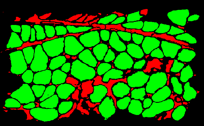
We can use the trained SVM to classify ROIs from a new file, and compare its predictions to predictions done by hand (manually marking ROIs as positives or negatives), to calculate our classifier's precision and recall.
Conclusion
The process of manually detecting and measuring muscle fibers is tedious and prone to measurement bias, yet most studies of muscle fibers continue to use this manual method. The field could greatly benefit from software that uses modern machine learning methods to automate this task. In this post I've presented my attempt to solve the problem. The code that implements it - myoquant - is open source and freely available. I warmly encourage other researchers to try it and see if they can use it or parts of it to solve their own lab-specific problems.