Introduction
Lately I've been playing around with this idea that concepts - the ideas behind the words in the dictionary - are the hidden causes behind a set of observed features. If we look up 'camel' in the dictionary, the entry reads: camel: "A large, long-necked ungulate mammal of arid country, with long slender legs, broad cushioned feet, and either one or two humps on the back." In my framework, when the hidden cause symbolized by the word camel is present, the features that are generated by the cause - long slender legs, broad cushioned feet, one or two humps - are all present. We mentally group the features that make up a camel into a singular concept because these features are highly correlated, and this correlation implies a hidden cause. The presence of the hidden cause is sufficient (but not necessary) to generate all the features of a camel.
If concepts are hidden causes of features, how do we detect them in the first place? How is it possible that we can look at an entity that has the features of a camel and immediately identify it as being a camel? I propose a model that looks something like this:
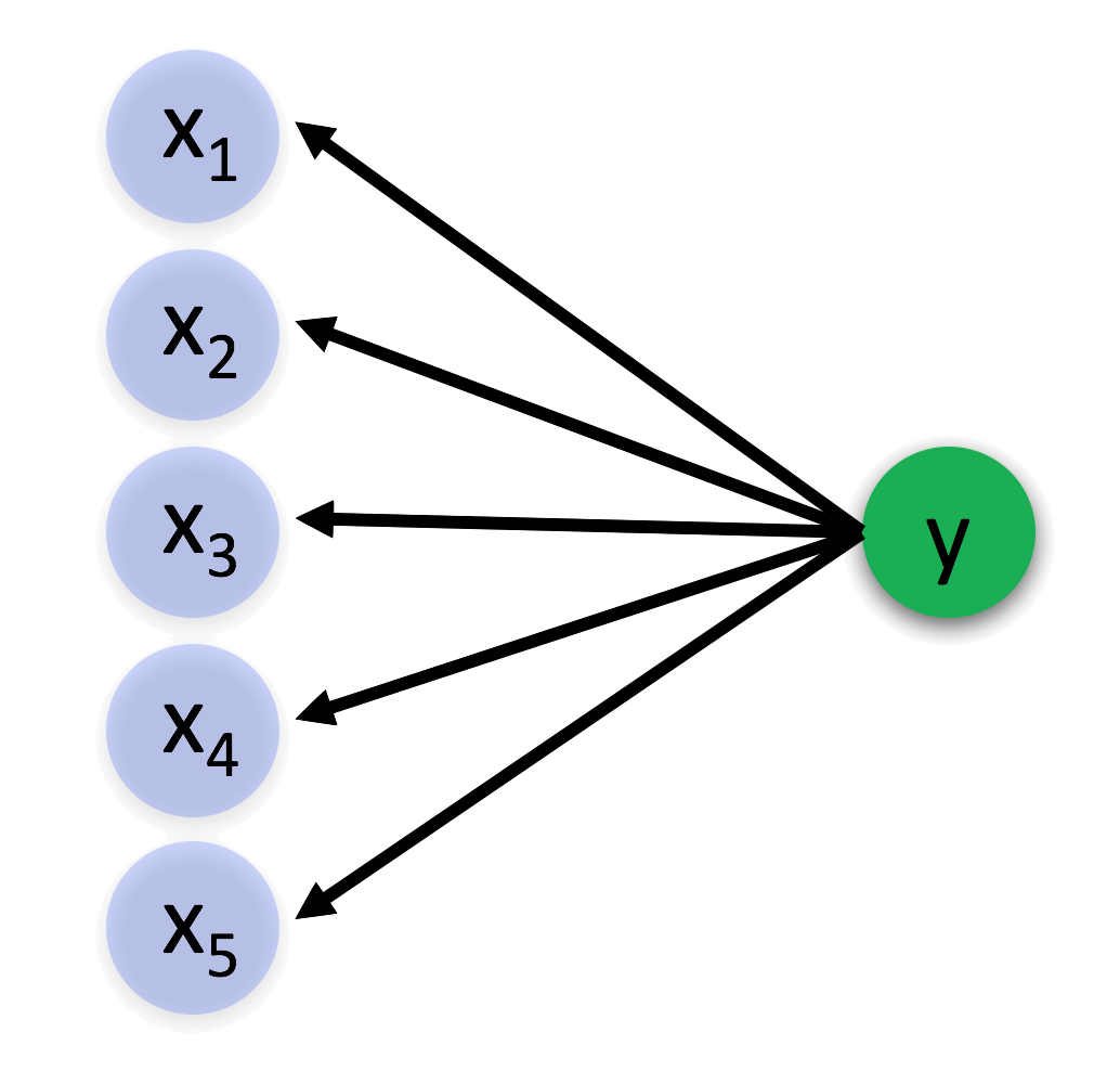
Where \(y\) is the hidden cause and \(\{x_1, x_2, x_3, x_4, x_5\}\) are the observable effects, or features of the concept. In this framework, concept formation is the process of determining that a set of features are so correlated that they are probably generated by a common hidden cause. Once we have learned the relation between the hidden cause and the features, then when we observe enough of the features to be present, we infer that the hidden cause is present. This is powerful because it then enables us to determine that the remaining features caused by the hidden cause must also be present.
What is the rationale for thinking that any correlated features we observe must have a hidden cause? If a set of features are highly correlated, and if the correlation is not spurious, there must be a reason they are correlated. Suppose the features \(\{x_1, x_2, x_3, x_4, x_5\}\) are correlated. This means that either a subset of those features cause the others, or that all of the features have some hidden cause. Once we have determined that there is a correlation between a set of features, we can group them together as a concept. Then when we observe some subset of the features, we can infer the probability of the hidden cause given a subset of the features, and predict the presence or absence of the remaining features.
Inferring a hidden cause
This post describes how to detect the presence or absence of a hidden cause which brings about the presence of a set of observable features. It also details the probability that the remaining features are present. More formally, the goal of this post can be stated: In a system of binary variables where a hidden variable causes the presence of all members of a set of binary features \(\{x_1, x_2, x_3, x_4, ..., x_n\}\), given the known presence or absence of a subset of the features, predict the probability that the remaining features are present.
To make this formalization a little more real, suppose we have 4 distinct coins. At the beginning of every trial, we throw all 4 coins together, each one comes up heads or tails, and we record the result. The coins aren't necessarily fair, and the probability that a given coin comes up heads is unknown to us. The coins are magnetic, and the table has a switch which controls its magnetism. When the switch is turned on, the table becomes magnetic, and all 4 of the coins come up heads with 100% probability. When the switch is turned off, the 4 coins come up heads with their normal probabilities, and the coins' values are uncorrelated. In this scenario, the hidden cause is the magnetism of the table. The only source of correlation between the coins is the hidden cause.
Once we have observed a large number of trials, after we throw the coins and before we can observe the result someone puts a piece of paper over some of the coins and asks you to guess whether they were heads or tails. Our goal is to determine the probability that each hidden coin is heads.
How should we get started? We probably want to determine the probability that the table is magnetized given the value of the coins that we can observe. Once we have that probability, we'll calculate the probability that a hidden coin is heads.
Let's generate some random binary variables. We'll call our 4 coins \(x_1, x_2, x_3, x_4\). Each coin's value will be 'True' or '1' if it is heads and 'False' or '0' if it is tails. We'll call the variable representing the magnetic table 'y', and it will be '1' when the magnetism is turned on and '0' when it is off.
import numpy as np
import matplotlib.pyplot as plt
import seaborn as sns
import pandas as pd
%matplotlib inline
sns.set(font_scale=2)
inv = np.invert # This function flips the bits in an array. We use it so often, we're creating an alias
def rbin(p, N):
    ''' Returns a random binary array of length N, where True values is present with probability p '''
    return np.random.binomial(1, p, N).astype(np.bool)
np.random.seed(31)
N = 100000
y = rbin(.2, N)  # y is the hidden cause
x1 = rbin(.5, N) * inv(y) + y  # When y is absent, P(x1) = 0.5. When y is present, P(x1) = 1
x2 = rbin(.6, N) * inv(y) + y
x3 = rbin(.8, N) * inv(y) + y
x4 = rbin(.5, N) * inv(y) + y

df = pd.DataFrame({'x1': x1.astype(np.int),
                   'x2': x2.astype(np.int),
                   'x3': x2.astype(np.int),
                   'x4': x2.astype(np.int),
                   'y': y.astype(np.int)})
df.head()
| x1 | x2 | x3 | x4 | y | |
|---|---|---|---|---|---|
| 0 | 1 | 1 | 1 | 1 | 0 |
| 1 | 1 | 1 | 1 | 1 | 1 |
| 2 | 0 | 1 | 1 | 1 | 0 |
| 3 | 1 | 1 | 1 | 1 | 1 |
| 4 | 1 | 1 | 1 | 1 | 0 |
If we could directly observe the hidden cause y, then when it is present we could infer with certainty that each feature \(x_1, x_2, x_3, x_4\) was present. However, y is hidden, so we can't directly use it.
If we had unlimited data, we could calculate the conditional probability of the unknown features being present given the known features. So if \(x_1\) was unknown, we could calculate its conditional probabilities given the known features:
print('P(x1) = {}'.format(x1.mean()))
print('P(x1|x2) = {}'.format(x1[x2].mean()))
print('P(x1|x2, x3) = {}'.format(x1[x2 * x3].mean()))
print('P(x1|x2, x3, x4) = {}'.format(x1[x2 * x3 * x4].mean()))
P(x1) = 0.5979
P(x1|x2) = 0.6446548277078679
P(x1|x2, x3) = 0.6705448937628513
P(x1|x2, x3, x4) = 0.755482764797707
However, if we know that the only feature causing the features to be correlated was the hidden feature y, we can break our estimation into two steps.
- First, we use the observed x's to estimate the probability that the hidden cause y is present.
- Then given our probability that y is present, we estimate the remaining parameters.
Step 1
If y is always hidden, how do we get \(P(y|x_1, x_2, x_3, x_4)\)? This is the tricky part. The only thing we know is that the probability of y increases as each feature is present. We know that whenever y is present, all \(x_1, x_2, x_3, x_4\) are present. This means that when any of them are absent, P(y) = 0. But sometimes all the features \(x_1, x_2, x_3, x_4\) can be present when y is absent. How often does this happen? Since all the features are independent when y is absent, the probability that they are coincidentally present when y is absent is the product of the probabilities they are present conditioned on y being absent.
We are trying to figure out \(P(y | x_1, x_2, x_3, x_4)\). According to Bayes rule:
Because $ P(x_1, x_2, x_3, x_4 | y) = 1 $ This reduces to
Expanding the denominator:
which equals:
Putting it together:
We can check this equation by measuring the estimations of these from our simulation.
left_side = y[x1*x2*x3*x4].mean()
print('Left side of the equation: {}'.format(left_side))
Left side of the equation: 0.6749881444346589
p_y = y.mean()
right_side = p_y / (p_y + x1[inv(y)].mean() * x2[inv(y)].mean() * x3[inv(y)].mean() *  x4[inv(y)].mean() * inv(y).mean())
print('Right side of the equation: {}'.format(left_side))
Right side of the equation: 0.6749881444346589
This suggests the equation is correct.
Solving for P(y|x)
There is only one free parameter in this equation, \(P(y | x_1, x_2, x_3, x_4)\). We can solve for it using our data with some algebra. Let's define some terms.
- \(N\) is the total number of observations or trials
- \(M_i\) is the number of times \(x_i\) was observed
- \(C\) is the number of times the conjunction of all x's was observed.
- \(p\) is our estimate for our free parameter, \(P(y | x_1, x_2, x_3, x_4)\)
Now our equation above becomes:
With some algebra:
N = len(x1)
allx = x1 * x2 * x3 * x4
C = np.sum(allx)
M1 = np.sum(x1)
M2 = np.sum(x2)
M3 = np.sum(x3)
M4 = np.sum(x4)
def loss(p):
    return (p-1) + (N/C - p) * \
            ((M1 - C*p) / (N-C*p)) * \
            ((M2 - C*p) / (N-C*p)) * \
            ((M3 - C*p) / (N-C*p)) * \
            ((M4 - C*p) / (N-C*p))
a = np.arange(0,1,.001)
b = np.array([loss(aa) for aa in a])
plt.plot(a, b**2);
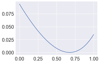
p_hat = a[(b**2).argmin()]
p_hat
0.676
allx = x1 * x2 * x3 * x4
y[allx].mean()
0.6749881444346589
import tensorflow as tf
def minimize_p():
    p = tf.Variable(0.5, trainable=True)
    loss = (p-1) + (N/C - p) * \
                ((M1 - C*p) / (N-C*p)) * \
                ((M2 - C*p) / (N-C*p)) * \
                ((M3 - C*p) / (N-C*p)) * \
                ((M4 - C*p) / (N-C*p))
    loss = loss **2
    opt = tf.train.GradientDescentOptimizer(1).minimize(loss)
    with tf.Session() as sess:
        sess.run(tf.global_variables_initializer())
        for i in range(30):
            #print(sess.run([p,loss]))
            sess.run(opt)
        result = sess.run(p)
    return result
p = minimize_p()
print(p)
0.67627406
Now that we've found \(P(y | x_1, x_2, x_3, x_4)\), we can easily calculate:
- \(P(y)\)
- \(P(x_1 | \neg y)\), \(P(x_2 | \neg y)\), \(P(x_3 | \neg y)\), \(P(x_4 | \neg y)\)
y_hat = x1 * x2 * x3 * x4 * p
p_y = (y_hat).mean()
noty_hat = (1-y_hat)
p_x1_given_noty = np.sum(noty_hat * x1) / np.sum(noty_hat)
p_x2_given_noty = np.sum(noty_hat * x2) / np.sum(noty_hat)
p_x3_given_noty = np.sum(noty_hat * x3) / np.sum(noty_hat)
p_x4_given_noty = np.sum(noty_hat * x4) / np.sum(noty_hat)

print('p_y: {}'.format(p_y))
print('p_x1_given_noty: {}'.format(p_x1_given_noty))
print('p_x2_given_noty: {}'.format(p_x2_given_noty))
print('p_x3_given_noty: {}'.format(p_x3_given_noty))
print('p_x4_given_noty: {}'.format(p_x4_given_noty))
p_y: 0.1996496468782425
p_x1_given_noty: 0.49759504199028015
p_x2_given_noty: 0.600475013256073
p_x3_given_noty: 0.7994753122329712
p_x4_given_noty: 0.4998815357685089
Step 2
Step 2 is much easier. Now that P(y) is determined, we can calculate the probability of the missing features with: $$ P(x_1) = P(x_1 | y) \cdot P(y) + P(x_1 | \neg y) \cdot P(\neg y) $$
\(P(x_1 | y) = 1\) because y causes \(x_1\) 100% of the time, so the equation reduces to
There are 3 terms in the right side of this equation. \(P(y)\) is what we get out of the first step, and it varies from trial to trial. \(P(\neg y)\) is \(1 - P(y)\).
$P(x_1 | \neg y) $ is the baseline probability of \(x_1\), generated by causes outside our system and assumed to be constant for every trial.
(see proof of calculation 1)
np.sum(inv(y) * x1) / np.sum(inv(y))
0.49783322718019807
def proof_of_calculation_1(x1):
    N = len(x1)
    p_y_given_x = .8
    p_y_given_not_x = .4
    y = np.zeros_like(x1, dtype=np.bool)
    py = np.zeros_like(x1, dtype=np.float)
    py[x1] = p_y_given_x
    py[inv(x1)] = p_y_given_not_x
    y[x1] = np.random.binomial(1, p_y_given_x, np.sum(x1))
    y[inv(x1)] = np.random.binomial(1, p_y_given_not_x, N - np.sum(x1))
    print(np.sum(py * x1) / np.sum(py))
    print(x1[y].mean())
proof_of_calculation_1(x1)
0.7483572188497403
0.749119869818967
Prediction
Now that we have all the important numbers from our training data, we can begin to make predictions. Suppose we only have a subset of x's, and we are trying to predict the remainder. If we observe \(x_2\), \(x_3\), and \(x_4\), we can determine the probability of the hidden cause:
p_y_given_x234 = p_y / (p_y + (1-p_y) * p_x2_given_noty * p_x3_given_noty * p_x4_given_noty)
print(p_y_given_x234)
0.5096819154029759
This is the probability of our hidden cause. We can use this to infer the probability of the remaining \(x\) in step two: $$ P(x_1) = P(y) + P(x_1 | \neg y) \cdot P(\neg y) $$
x1hat = p_y_given_x234 + p_x1_given_noty * (1 - p_y_given_x234)
print("Prediction of x1 given the probability of y = {}".format(x1hat))
Prediction of x1 given the probability of y = 0.7536617632966258
print('P(x1|x2, x3, x4) = {}'.format(x1[x2 * x3 * x4].mean()))
P(x1|x2, x3, x4) = 0.755482764797707
This is the prediction that we got without using y at all, when we have large numbers.
Discussion
The results above have shown that given any row of incomplete data, we can use a few assumptions to fill it in. The assumptions are
- There is a hidden cause that, when present, causes all the features to be present.
- When the hidden cause is absent, the presence of any feature is independent of all the others.
Both of these assumptions are strong and perhaps unrealistic. Suppose we have two causes c1 and c2, each independent of each other, but which impinge upon common effects \(x_1\) and \(x_2\). Assumption 2 would be violated, because when c1 is absent, \(x_1\) and \(x_2\) are dependent via c2.
However, the situation might be rescued by supposing that there is some third cause c3 by which both c1 and c2 act to bring about effects \(x_1\) and \(x_2\).
Then we can say that c3 is the effect of c1, rather than \(x_1\) and \(x_2\). Because all c1's features are independent, assumption 2 is satisfied.
It should be possible to create a complicated causal network. By repeatedly observing the features, we can build up a network of hidden causes. Once we have constructed this network, when we make observations we can 1) infer the presence of the hidden causes and use those to 2) predict the probabilities of the remainder of hidden features which have not been observed.
Analogy via abstract concepts
Once we have built up this structure, we can do more complicated inferences. Specifically, we can reason by analogy. Suppose we have two causes c1 and c2, which have some overlapping effects
Suppose we have another cause c3 and we are aware of some of its effects.
c3's effects have an analogous structure to c1's and c2's. All three cause \(x_3\) and \(x_4\). We could make an inductive leap and assume c1, c2, and c3 bring about another hidden cause - \(c_4\) - which causes \(x_3\) and \(x_4\), and perhaps also \(x_5\)
This is an inductive inference and isn't certain, but if this causal structure were true we would conclude that when \(c_3\) is present, \(x_5\) is present, even if we never observed the correlation between \(x_5\) and the other effects of \(c_3\). We formed the abstract concept \(c_4\) that enables us to do inferences that wouldn't have been possible otherwise.
This inference is powerful because it allows transfer learning. We can learn some causal substructure that holds true no matter where it is found, including in novel hidden causes (or concepts). We don't have to determine the correlation from scratch every time.
Discovering and modeling these 'middle' hidden causes also protects our algorithm's assumption that the inputs are uncorrelated in the absence of the hidden cause.
Modus ponens
Suppose we know that a cause \(c\) implies an effect \(x_1\). Then when we determine the cause is present, we can validly conclude that the effect is also present.
As an example, suppose we know that all men are mortal. That is, for any entity that contains all of properties of being a man (having DNA of homo sapiens, breathing oxygen, eating food, etc.), we can be certain that that entity has the property of being mortal. In the algorithm presented above, there are two steps: 1) determining the relationship between the features and the hidden cause, and 2) inferring the remainder of the features given a subset of them by determining the probability of the hidden cause. In this case, our 'hidden cause' of mortality is the state of being a man. In other words, being a man causes mortality. We can be certain of this through inductive generalization: we observe a million entities that all have correlated features \(x_1\), \(x_2\), ..., \(x_n\). One of these properties is mortality, and we infer that the hidden cause that makes these properties probabilistically dependent is \(y\): being a man. Now that we've determined the probabilistic relationship between the features and the hidden causes, when we see an entity walking down the street wearing a name tag that says "Hello my name is Socrates", by using the subset of features that are caused by the hidden cause, we determine the probability that the entity before us is a man. If we observe lots of properties, and \(P(\neg y|x_1, x_2, x_3,...)\) is very low, we conclude with high certainty that the entity is a man. The deductive step immediately follows: because all men are mortal, and this is a man with high probability, then this is mortal with high probability.
If $\forall x(Ax \implies Bx) $, then we can think of A as being the entirety or part of a hidden (sufficient) cause for B.