Introduction
Gradient boosting is one of the most powerful and widely used machine learning algorithms as of this writing. In this post, we will look at gradient boosting and the intuition behind it. The syntax follows the excellent series of posts at explained.ai.
Decision Tree Regression
There are many machine learning models that can predict a target variable given a set of input features. Decision trees are one of the simpler models, and form the basis of most implementations of gradient boosting. Before we get into gradient boosting, let's see how decision trees are trained and how they infer target variables.
Training
Decision trees take the training data and split it repeatedly according to the value of a particular feature. At each split ('branch point' in the tree metaphor), the data is divided into two branches: left and right. The feature and the threshold to split are chosen so they separate the data in the best way. For regression, the 'best' split is usually the split (feature and threshold combination) that minimizes the variance in the training data in each of the two branches. Each branch is then split again, and again, until some stopping criteria. Once this stopping criteria is reached, no more branches are created, and the data is put into a leaf.
Inference
Once the model is trained, a new data point is passed into the decision tree. It starts at the root, and gets routed to the left or right branches depending on the learned criteria (feature/threshold combination) at that branch point. Once the data point gets to a leaf, a prediction is issued as the mean value of the training data that defined that leaf.
Here is my implementation of a decision tree regressor:
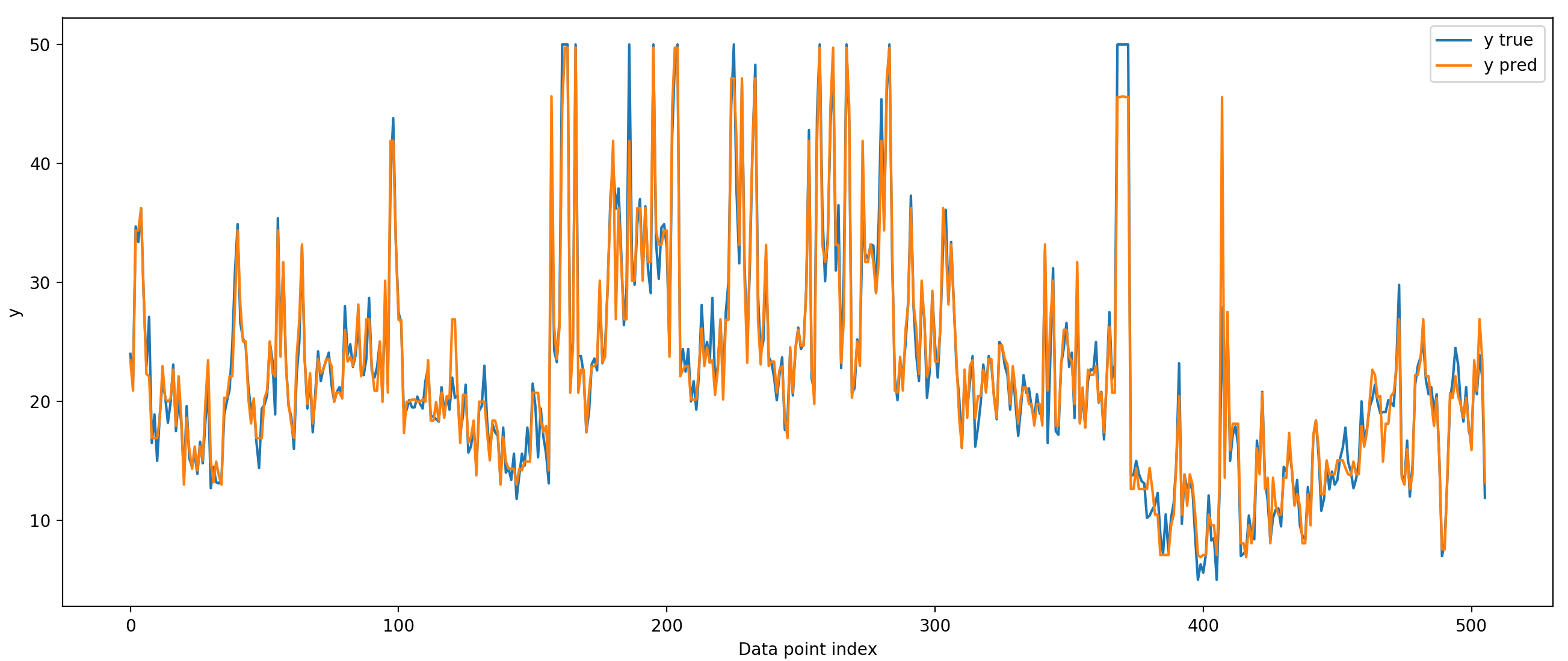
In the script above, training and testing are on the same data, so we wouldn't expect the model's performance to generalize to other data sampled from the same distribution. We are overfitting to the training data because we are allowing the tree to be very deep (have lots of branch points). We can prevent this overfitting by reducing the depth of the tree. We can even make 'stumps' - decision trees with only one branch point. These small trees are called weak learners because each one of them has high bias; they will have high error because they can't fit complicated functions. However, if we chain several of these weak learners together, we can make an extremely good model. This is the reasoning behind boosting in general, and gradient boosting in particular.
Chaining Decision Trees
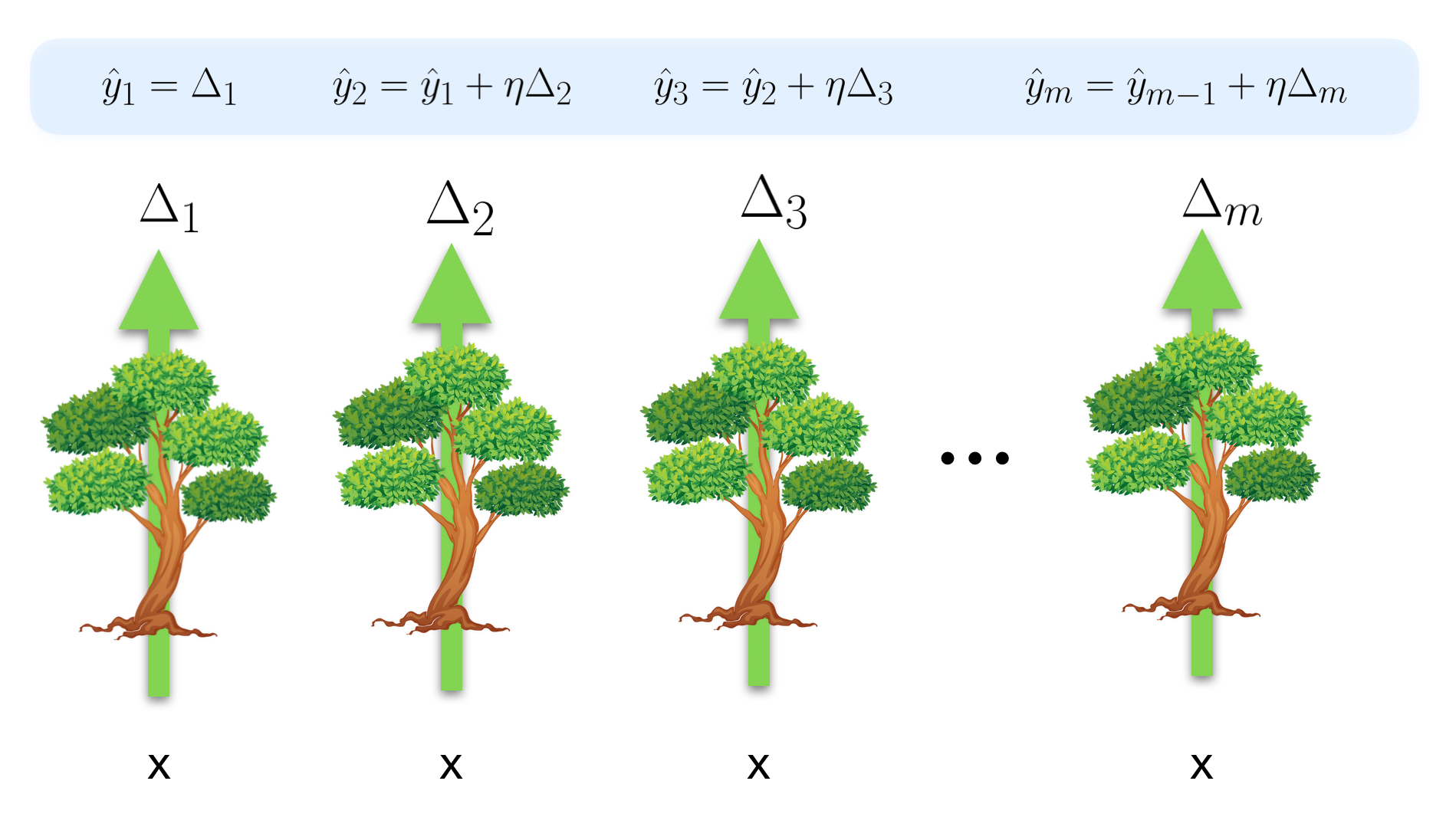
In gradient boosting, during inference each tree takes the input features and outputs a number, but this number isn't a direct estimate of the target variable. Instead, it is an estimate of the gradient that points in the direction we need to go in order to correct the output generated by adding up all the previous trees' predictions. In other words, at each tree we generate a prediction, and the next tree corrects that prediction by adding a delta which depends on the input features.
What is the loss function each tree is trying to minimize? Let's formalize the concept of how wrong we are in our prediction after the \(m\)th tree. For each point in our training data, after each tree generates an output, we will have a prediction \(\hat{y}\) and a true target value \(y\). If we have \(N\) points in our training data, then our true and predicted target values form a vector of length \(N\). We can take the difference between the true value and the predicted value to get a residual vector \(\boldsymbol{r}\_m = \boldsymbol{y} - \boldsymbol{\hat{y}}\_m\). If we are doing regression with MSE loss, then each tree is trying to find the features and thresholds which best approximates the residual vector from the previous step. That is, each tree is trying to minimize the difference between its output \(\Delta_m\) and the previous residual vector \(\boldsymbol{r}\_{m-1}\), as measured by some loss function (e.g. squared error) \(\mathcal{L}_{se}(\boldsymbol{r}\_{m-1}, \Delta_m)\). If a tree succeeds completely, then \(\Delta_m = \boldsymbol{r}\_{m-1}\), and if the learning rate \(\eta\) is 1, the new residual becomes \(\boldsymbol{r}\_m = \boldsymbol{0}\).
Gradient in prediction space
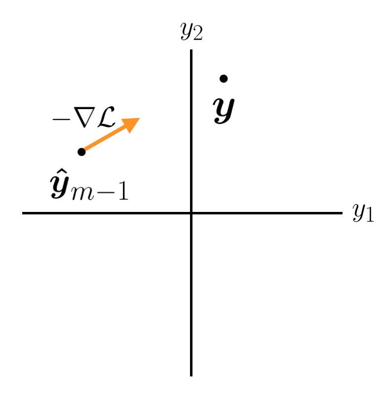
There is another, more general way to think about the function we are trying to minimize at each step. Let's imagine we have a point in our target space that we are trying to get to, located at \(\boldsymbol{y}\). The dimensionality of this space is the number of points we have in our training data. After the \(m\)th tree, we have a prediction \(\boldsymbol{\hat{y}}\_m\). We want this point to get closer to \(\boldsymbol{y}\).
Ideally we would like the next tree to cause the prediction to jump exactly to the true \(\boldsymbol{y}\). And we could do this with a high capacity model. However, we are using weak learners with low capacity in order to prevent overfitting. A high bias, weak learner is probably not going to cause our overall model to move directly to \(\boldsymbol{y}\). The next best thing is moving in the correct direction. However, we are forced to make a tradeoff. We can improve the prediction for some data points but this improvement will be at the expense of other data points. If we have N points, maybe we can make the first prediction perfect, but this would cause all the other predictions to be even worse off than before this stage. This is obviously not good. What principled way can we use to decide which \(y\)s to prioritize?
We can imagine that our weak learner is only going to allow us to move our \(\boldsymbol{\hat{y}}\_m\) vector an infinitesimally small distance. Which direction is the best? At every point in our prediction space we have a loss. If our loss function is MSE, then that loss is the square of the distance away from \(\boldsymbol{y}\), and is equal to zero at \(\boldsymbol{y}\). The direction in which we could change our \(y\) predictions where we would get the best improvement in our overall loss function is given by the negative gradient of our loss function in prediction space: \(-\nabla \mathcal{L}\). This suggests that the best we could hope to improve our model is by using a weak learner that does its best to predict the negative gradient \(- \nabla \mathcal{L}\), and then we can move some distance \(\eta\) along that gradient to generate our new prediction \(\boldsymbol{\hat{y}}\_m\). This is in fact what gradient boosting does.
Each tree is searching over its parameters to find the output \(\Delta\_m\) which best estimates \(- \nabla \mathcal{L}\). Let's see what this looks like for the MSE loss function.
MSE Loss
Let's evaluate the gradient for the MSE loss to see what function each regression tree should attempt to approximate.
This result states that the function the \(m\)th tree is trying to estimate is 2 times the residual from the previous stage. (In practice the constant factor of 2 is absorbed into the learning rate \(\eta\) — equivalently, define the loss with a factor of \(\frac{1}{2}\) so the negative gradient is exactly the residual — so the tree just fits the residual.) In other words, our decision tree should do its best to estimate the difference between where we want to be and where we are. This is what we stated above, and matches our intuition well. As we said above, if our model outputs \(\Delta\_m = \boldsymbol{r}\_{m-1}\), then we will be fitting our training data perfectly at this stage.
Other loss functions
This same procedure works for any differentiable loss function. The output of the previous tree will give us \(\boldsymbol{\hat{y}}\_{m-1}\). We can compute the direction that most rapidly decreases our loss function by taking the gradient of the loss function in prediction space, evaluated at \(\boldsymbol{\hat{y}}\_{m-1}\). This will point us in the direction that is most likely to give us an improvement in our model. Then we find the parameters of the \(m\)th tree that get us as close to this gradient as possible. We then move \(\eta\) distance along that gradient to a new location which will (usually) be closer to \(\boldsymbol{y}\) than the previous estimate.
This entire procedure is called gradient descent in function space. The term 'function space' is the same as what we've been calling prediction space, and is so called because the space we are moving in is made up of the \(N\) values of the \(\hat{y}\)s, which are outputs of the chain of trees. The term 'gradient descent' is used because the direction we are moving in is the negative gradient of the loss function in this prediction space. This is very different to the usual gradient descent in parameter space that is common to many machine learning models, including neural networks. Although we are finding the parameters of the individual models that minimize the loss (and in fact we could use gradient descent in parameter space to accomplish this), the tree-specific target we are trying to fit changes from tree to tree: it is the negative gradient of our global loss function in prediction space, evaluated at where the previous tree left us.
Conclusion
In this post we saw how gradient boosting works. In another post we will look at how this same framework can be used to perform classification, by changing the loss function.