I've been reading about the potential-outcomes model, which enables you to determine how much a treatment affects a unit. A unit is a particular entity, like a patient. A treatment is a feature of that unit that can potentially be set, like a doctor giving a patient a drug. For a given unit, we would like to know how much a treatment would affect another feature of the unit, like whether or not they have a cough. This feature is called the response variable.

The problem would be easily solved if we could copy that unit exactly, and we give the treatment to one and not to the other. The causal effect would simply be the difference between the response in the treated unit vs the untreated unit. However, we can't make perfect replicas of many units, like people or countries. But we still would like to know the causal effect of a treatment. So how can we do this?

The answer is to try to infer what would have been the effect had we done the treatment, for the units we don't give the treatment, and vice versa. These are called potential outcomes. For a given unit you can't observe both potential outcomes, but if you can use information about units that are similar to each other, you can infer what both potential outcomes probably would be.

Suppose the only factors that matter in whether or not someone with SARS-CoV-2 will go on to develop symptoms are their age, how many hours a week they work out, and if they breathe clean air. And suppose that relationship between those three features and the binary response of developing symptoms was perfectly deterministic. Then, if we wanted to know whether breathing clean air would prevent a 55 year old who works out 5 hours a week would prevent symptoms compared to breathing polluted air, we just have to find 55 years olds who work out 5 hours a day from polluted and unpolluted regions and see if they have symptoms. Then we would have our answer. Since the geographic region of the patient does not causally affect whether or not the patient has symptoms (given the 3 relevant features), we would not need to find patients from the same region. We can ignore that variable.

The crux of using the potential effects model, and the real trick of causal inference, is grouping units by similarity and then assuming the causal effects are the same among similar units. The main difficulty becomes determining which units are similar with respect to the response variable. This is not trivial. The question we need to answer is essentially: which features of units will change the relationship between the treatment and the response? Some features are completely unrelated. In the disease example, the third letter of the patient's first name doesn't matter at all, although that is a feature of the patient. Some features, like age, are extremely relevant and should definitely be used to determine similarity.

The backdoor path criteria (Pearl, 2000) provides a solution, but requires some strong assumptions. If you know the causal graph of conditional dependencies between features of a unit, then the features you need to use to stratify/condition on in order to compare similar units to each other are simply the features which close all backdoor paths connecting the treatment C to the response E. This post explores that idea with simulated data.

import numpy as np
import matplotlib.pyplot as plt
import seaborn as sns

# Plotting
from pandas.plotting import register_matplotlib_converters
register_matplotlib_converters()
sns.set_context("notebook", font_scale=1.3)
sns.set_style("darkgrid")
%config InlineBackend.figure_format = 'retina'

blue_d = '#0044BD'
blue_l = '#67A2FF'
red_d = '#BE0004'
red_l = '#ED686A'

def plot_C_given_B(B, C, P_C_given_B=None):
    fig, ax = plt.subplots(figsize=(8, 3))
    ax.set_xlabel('B')
    ax.set_ylabel('P(C)')
    ax.plot(B, C, '.', label='C');
    if P_C_given_B is not None:
        ax.plot(B, P_C_given_B, '.', label='P(C)');
    ax.legend();

def plot_E_given_B(B, C, E):
    fig, ax = plt.subplots(figsize=(8, 3))
    ax.plot(B[C==0], E[C==0], '.', c=blue_d, label='E | C=0');
    ax.plot(B[C==1], E[C==1], '.', c=red_d, label='E | C=1');
    ax.set_xlabel('B')
    ax.set_ylabel('E')
    ax.legend();

def plot_E_given_C(C, E):
    fig, ax = plt.subplots(figsize=(5, 5))
    sns.boxplot(y=E, x=C, ax=ax, color=blue_l)
    ax.set_xticks(ticks=(0, 1));
    ax.set_xlabel('C')
    ax.set_ylabel('E');
    sns.swarmplot(y=E, x=C, ax=ax, color=blue_d);

def plot_E_given_B_2subplots(B, C, E):
    fig, (ax1, ax2) = plt.subplots(2, 1, figsize=(8, 7), sharex=True)
    ax1.plot(B[C==0], E[C==0], '.', label='C=0');
    ax1.set_ylabel('E | C=0')
    ax2.plot(B[C==1], E[C==1], '.', c=red_d, label='C=1');
    ax2.set_xlabel('B')
    ax2.set_ylabel('E | C=1')
    fig.legend();

Data Generation

Here we have three relevant variables. C is the treatment variable, or 'cause'. E is the response, or 'effect'. B is a background variable that is relevant to the relationship. I is an irrelevant feature of the units that is causally independent.

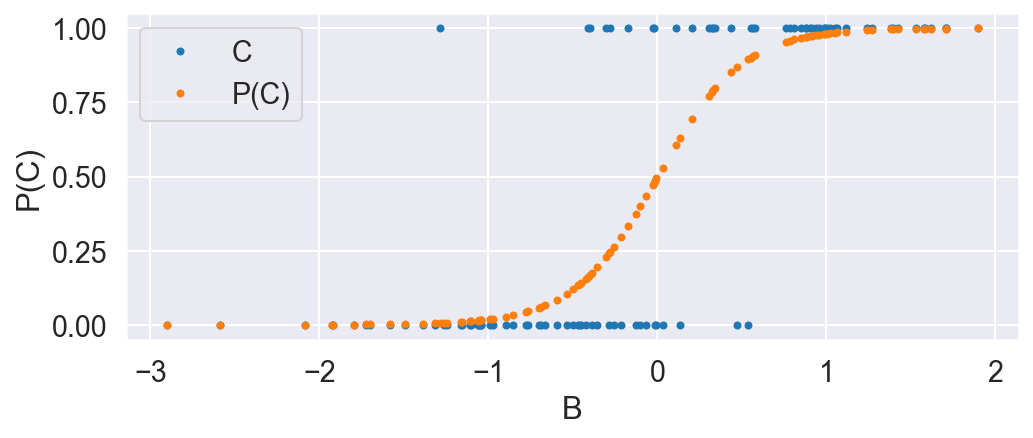
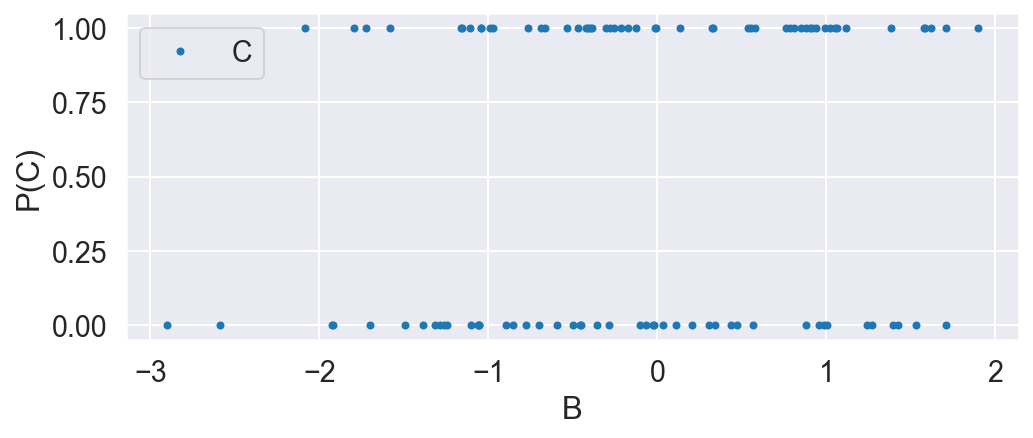
B is normally distributed. C is distributed according to the bernoulli distribution, where the probability is dependent on B according to the logistic function. This means the treatment group is enriched when B is high.

N = 100
np.random.seed(30)
B = np.random.normal(0, 1, N)
P_C_given_B = 1 / (1 + np.exp(-4 * B))
C = np.random.binomial(1, P_C_given_B)
plot_C_given_B(B, C, P_C_given_B)

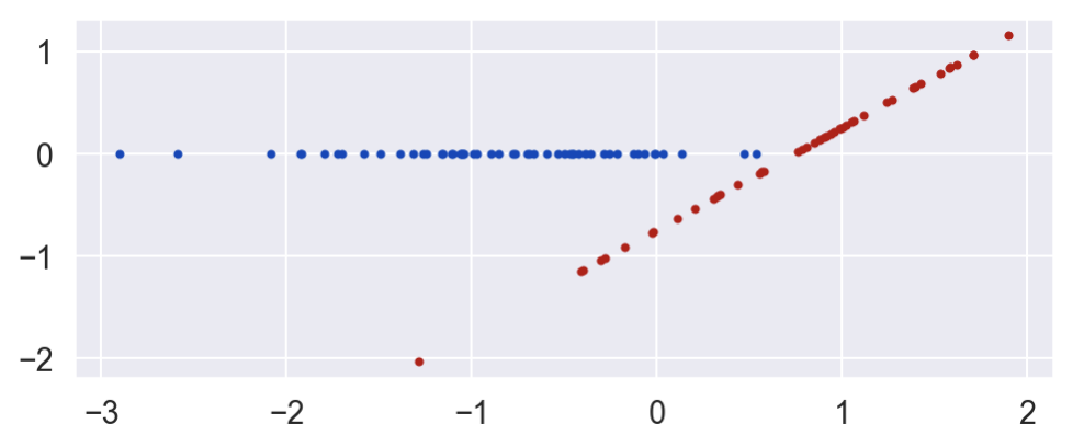
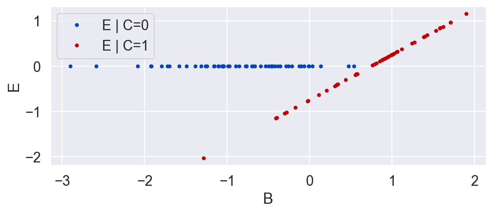
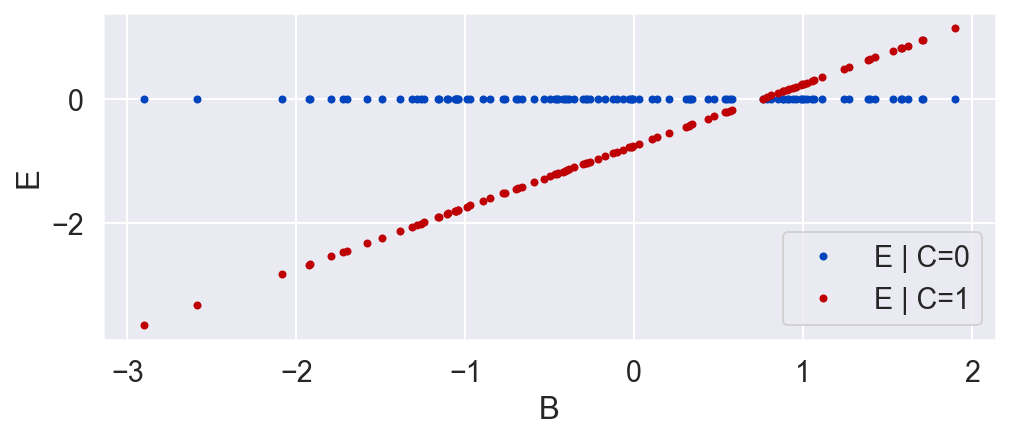
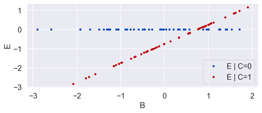
E's value is a deterministic function of B and C. E is 0 if the unit is in the control group (C=0) and is equal to B minus a constant when the unit is in the treatment group.

E = C * (B - .746)
plot_E_given_B(B, C, E)

Inference

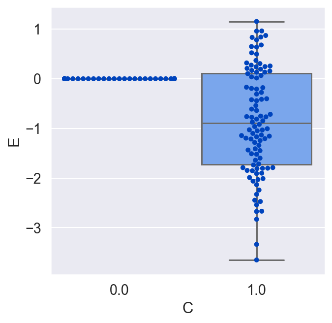
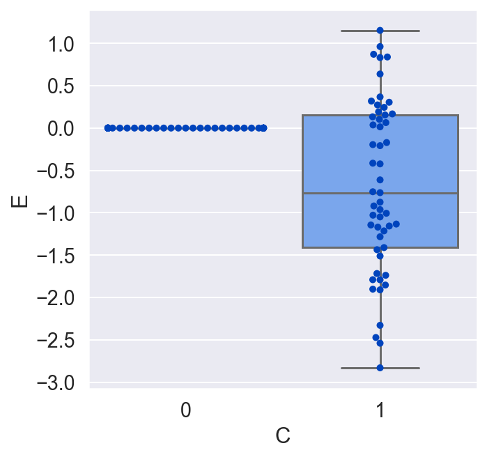
Suppose we were unaware of the background variable B, and we only wanted to look at the causal effect of C on E. C is binary, so we would look at E when C is 1 and again when C is 0.

plot_E_given_C(C, E)

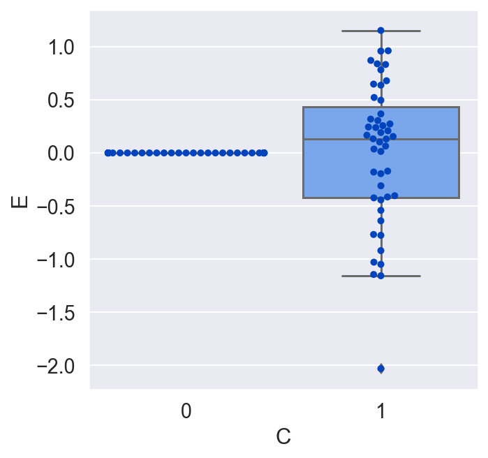
We would conclude that C has no effect on E on average, which is incorrect. Let's redo the plot, but this time let's make a copy of all the units, switch their treatment, and see what the average causal effect would have been for all the units. By doing this, we are actually doing that counterfactual test we would love to do in the real world but never can.

B2 = np.concatenate((B, B))
C2 = np.concatenate((np.ones_like(B), np.zeros_like(B)))
E2 = C2 * (B2 - .746)
plot_E_given_B(B2, C2, E2)
plot_E_given_C(C2, E2)

Now that we see the true causal effect for every unit, the average causal effect is negative, whereas before it was zero! What went wrong?

We ignored the fact that the effect E is dependent on B. Specifically, the value of E is linearly related to B if C equals 1.

In order to account for this we need to condition on B. Conditioning blocks the backdoor path from E to C through B. To do this, we pull B into our set of covariates $X$, and generate two response surfaces over X:

$$E_0 = f_0(X | C=0) $$ $$E_1 = f_1(X | C=1) $$

If we can fit these two functions, then we can determine what the causal effect C has on E for any particular value of X, by taking the difference between the two functions evaluated at X.

plot_E_given_B_2subplots(B, C, E)

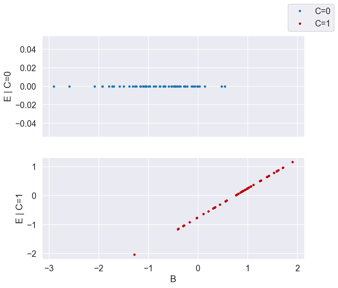
Now that we've stratified by C, the relationship between X (which in this case is B, since that's the only variable required to close all the backdoor paths between C and E), and E becomes clear. We can model $f_0$ and $f_1$ each with a straight line.

Then, if we'd like to determine the causal effect of C on a new unit that has a background variable B, we can evaluate the two functions at X and take their difference:

$$ \mathrm{Effect}_i = f_1(X_i) - f_0(X_i) $$

Randomized Experiments

If we didn't know the value of B, or that it created a backdoor path between C and E, we could remove its confounding effects by conducting a controlled experiment. This would break the causal link between B and E. Let's look at the data we would get from this.

C = np.random.binomial(1, .5, N)
plot_C_given_B(B, C)

E = C * (B - .746)
plot_E_given_B(B, C, E)

plot_E_given_C(C, E)

Now we conclude that C has an effect on E, and that on average, in the population we used in the randomized experiment, the effect of E on C was negative. While this is true, it is a much weaker conclusion than we had when we included B. While the causal relationship from E and B to C had been deterministic, the relationship from E to C without B is stochastic. That is, for a given unit, we can only get a probability distribution over the causal effect. And while on average the relationship is negative, for a given unit the impact of E on C might very well be positive! We just don't know, and we can't know, unless we include B and uncover the true deterministic relationship E = f(C, B).

To make matters worse, if someone conducts the same randomized experiment, but with a population of units that have different values for B. Let's run that experiment and see what happens.

B = np.random.normal(3, 1, N)
C = np.random.binomial(1, .5, N)
E = C * (B - .746)
plot_E_given_B(B, C, E)
plot_E_given_C(C, E)

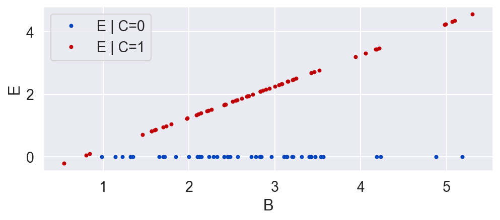
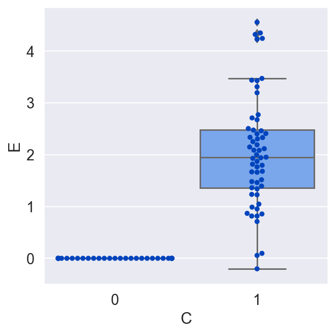
Whereas in our previous randomized experiment the average causal effect was negative, now, in a different randomized experiment the result is flipped. This is a paradoxical result. C now has a positive effect on average. This is all because E depends on B, which has a different distribution in each of the studies (B's mean was 0, and now it is 3).

Randomized experiments are useful for determining some aspects of causal links. For instance, if you do see a statistically significant average effect, you can conclude that there actually is a causal effect between the variables, and you know the direction of the arrow. But if you want to generalize those effects to a wider population of units, or turn a stochastic relationship into more of a deterministic one, you need a causal model that includes all the variables which causally interact to set the value of the response variable.

Conclusion

In the beginning of this post, I said that finding similar units with respect to the response is the main trick that enables us to measure causal effects. In the example, if two units had similar values of B, then they would have similar causal effects. In general, we want to come up with a list of features of the units such that if we take all the units that have identical values of those features, then the distributions of the potential outcomes should be the same among those units, for the units in the treatment and the units in the control. If we find 100 units that have identical values for those features that are ‘important’, then all those 100 units will be at the same point X in the domain of our response functions. If 70 of them get the treatment and 30 are in the control, then we can get an estimate of the average causal effect just by taking the average of the 70 minus the average of the 30. But this only works if, 1) had we given the treatment to the 30, they would have had the same distribution of outcomes as the actual treatment group, and 2) had we put the 70 in the control group, they would have had the same distribution of outcomes as the actual control group. The probability distribution of both potential outcomes over the response variable should be independent of whether or not they were actually placed in the treatment group, at a given point X. So our nebulous concept of ‘similarity between units with respect to the response’ can be quantified as how far apart they are in the feature space constructed using those variables we need to condition on.

When can you ignore a background variable?

If a background variable B is causally upstream of C but doesn't influence E (there is no backdoor path through B) then you can safely ignore it.

If a background variable mediates the link between C and E, then conditioning on it will break the link and lead you to the wrong conclusion that there is no causal relationship between C and E. This is post-treatment bias. Do not condition on a mediator.

If a background variable is downstream of C and E, then do not condition on it! This is called collider bias can easily lead you to believe that C influences E when it doesn't.

When should you include a background variable in the domain of your response function?

If a background variable influences E but has no impact on C, you can ignore it without leading you to the wrong conclusion, but as we saw in the randomized experiment case above, including B in the set of covariates you include in the domain of your response function would improve your understanding of the response surface.

Finally, as we've seen, if you have a common cause that opens a backdoor path between C and E, you should include it, to close the path.