KL Divergence Background

Suppose there is a true generative distribution $P$ and an agent that approximates this distribution with $Q$. The Kullback-Leibler (KL) divergence can be interpreted as the average relative surprise the agent will experience. This definition can be built up in three stages: 'surprise', 'relative surprise', and 'average relative surprise'.

Surprise

Intuitively, the surprise is a measure of the probability of observing a sample, that goes up as the probability of the sample goes down. We would like it to have the property that if we have two independent events, the surprise of the 'event' of observing both is the sum of their individual surprises. Per the rules of probability, the probability of observing two independent events is the product of their individual probabilities. Taken together, these desiderata are satisfied by the logarithm function.

\[ \begin{align} \text{Surprise } P(x):= -\log_2 P(x) \end{align} \]

If you're curious what happens in the continuous case when the probability density function exceeds 1 and the surprise becomes negative, see the side note below.

Relative Surprise

The relative surprise is the difference between the surprise that the agent expects from a sample and the surprise it should expect if it had a perfect model of the true generative distribution. That we have a quantity we're interpreting as the 'expected surprise' is counterintuitive; if an agent expects to be surprised, is it really surprised? It makes more sense when we think about aggregating many samples at a particular point in the sample space. If the agent knew the true distribution, it will be surprised by samples coming from a low probability region, so in this sense it is expecting to be surprised by those samples. But if there is a mismatch (divergence) between the agent's model and the true distribution, the agent will be more or less surprised by these samples than it would be if it knew the true generative distribution.

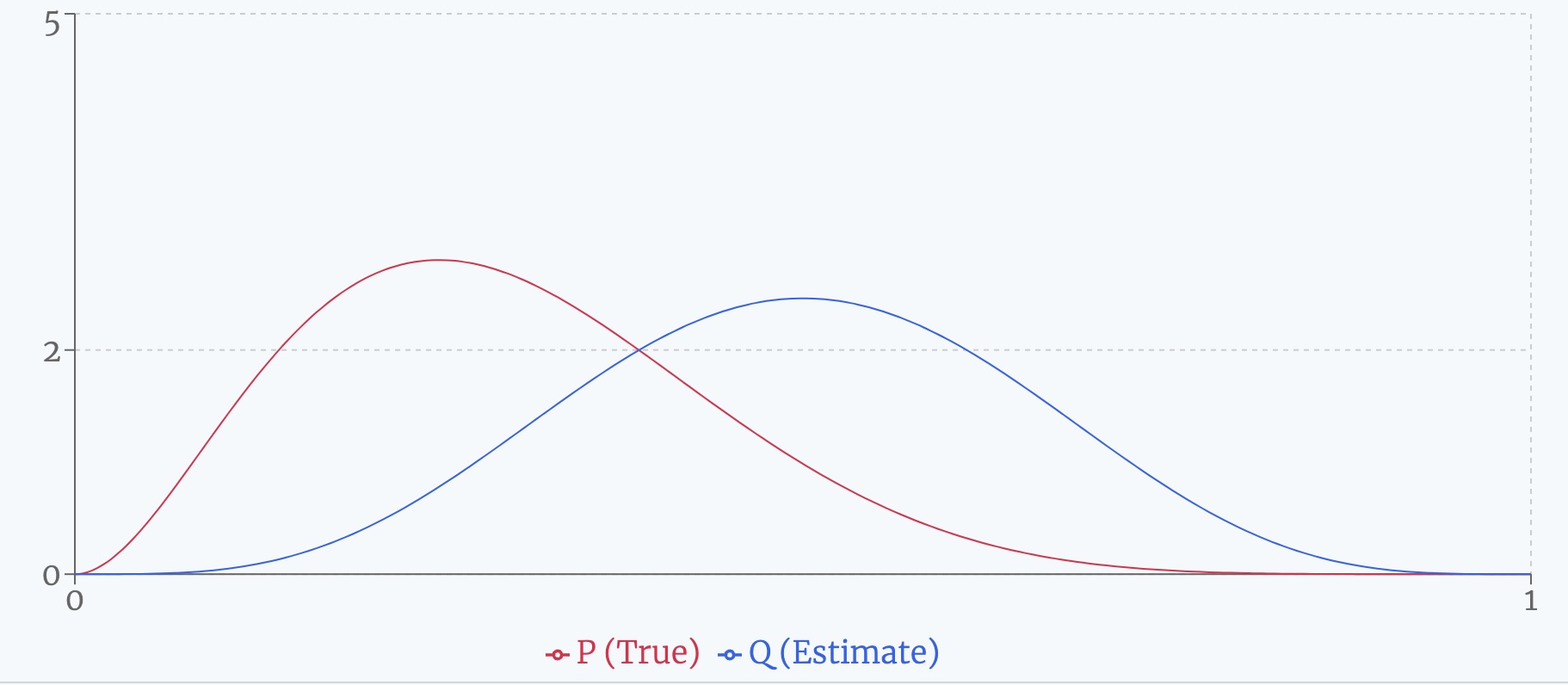
Suppose we have two beta distributions, as shown below, representing the true generative distribution and the agent's current approximation respectively. Then intuitively, the relative surprise is how much more surprised the agent is when observing a sample at $x$ than it ought to be. Algebraically:

\[ \begin{aligned} \text{Relative Surprise } P(x) || Q(x) &:= \text{Surprise } Q(x) - \text{Surprise } P(x) \\\ &= -\log_2 Q(x) - ( -\log_2 P(x)) \\\ &= \log_2 \frac{P(x)}{Q(x)} \end{aligned} \]

In the figure below, the individual surprises for two beta distributions are shown, as well as their relative surprise. In the bottom plot, each surprise is weighted by the probability of actually encountering that sample (i.e. $P(x)$). As discussed below, the integrals of these weighted surprises are the entropy, cross entropy, and KL divergence respectively. (For an explanation of why surprise and entropy can be negative, see the side note.)

Average Relative Surprise: KL Divergence

To measure how well $Q$ approximates $P$ overall, we can weight the relative surprises by how often the agent will encounter them. In other words, we should weight by $P(x)$. This is shown as the dotted green line in the plot below. Then, we can integrate over the entire sample space to get the 'average relative surprise', which is the Kullback-Leibler (KL) divergence.

\[ \begin{align} D_{\mathrm{KL}}(P || Q) &:= \int_{\mathcal{X}} P(x) \log \left( \frac{P(x)}{Q(x)} \right) dx \\\ & = \int_{\mathcal{X}} P(x) \bigg[ \text{Surprise } Q(x) - \text{Surprise } P(x) \bigg] dx \\\ &= \text{Average Relative Surprise} \end{align} \]

When Q matches P perfectly, the relative surprise is zero, so the KL divergence is zero. When Q underestimates P in regions where P has substantial probability mass, those regions contribute positively to the integral, increasing the KL divergence. On the other hand, when Q overestimates P, the agent has underestimated the surprise, so this brings down the KL divergence. However, since this underestimated surprise is less experienced by the agent, it contributes less. Taken together, the positive regions outweigh the negative regions, and the KL divergence can never be negative. The only time it is zero is when the agent's estimate of $P$ is perfect.

Putting it all together

This blog post has been mostly concerned with pointwise (pre-integration) concepts of probability distributions: weighted surprise and weighted relative surprise. When we take the expected value of these quantities with respect to some 'true' probability distribution $P$, we get entropy, cross-entropy, and KL divergence. Their relationship can be summarized with the following simple equation:

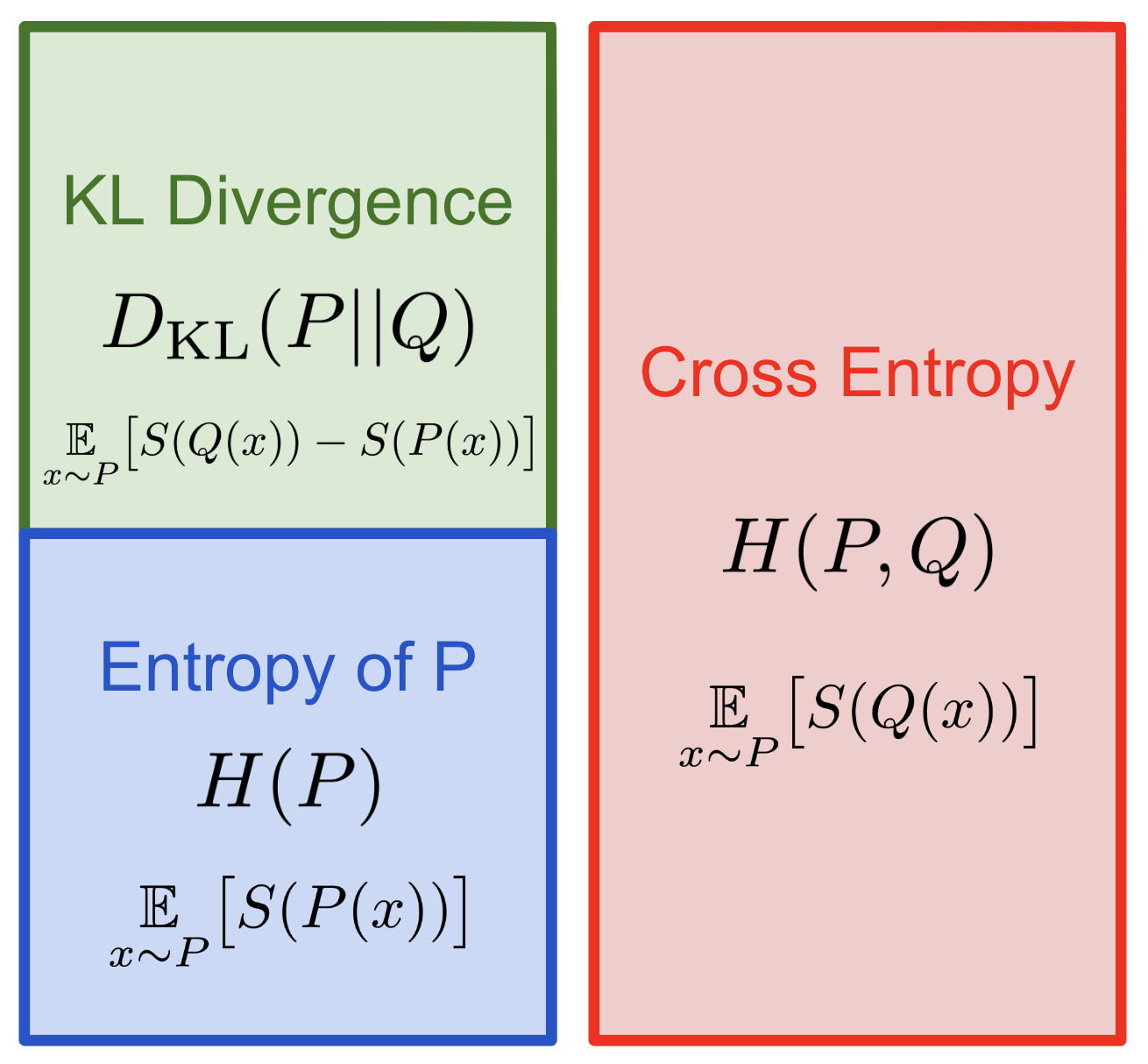
\[ \begin{array}{ccccc} \underset{x \sim P} {\mathbb{E}} \big[S(P(x))\big] & + & \underset{x \sim P} {\mathbb{E}} \big[S(Q(x)) - S(P(x))\big] & = & \underset{x \sim P} {\mathbb{E}} \big[S(Q(x))\big] \\ \text{Entropy} & + & \text{KL Divergence} & = & \text{Cross Entropy} \\ H(P) & + & D_{\mathrm{KL}}(P || Q) & = & H(P, Q) \\ \end{array} \]

If we imagine that $Q$ is an agent's mutable model and $P$ is the true, immutable generative distribution that $Q$ seeks to approximate, then the following are equivalent ways of getting $Q$ closer to $P$:

Minimizing cumulative surprise
Minimizing KL Divergence
Minimizing cross entropy

Subjective Logic

A lot of the inspiration for this post came from this Opinion Visualization Demo, created by Gaëtan Bouguier. This demo visualizes the correspondence between opinions in Audun Jøsang's Subjective Logic framework, and beta distributions. In my post, I used precision as one of the parameters for the beta distribution, where precision is the inverse of the variance of the beta. Given the two usual parameters $\alpha$ and $\beta$, the precision is given:

\[ \begin{align} \text{precision} &:= \frac{1}{\text{variance}} \\\ \text{precision} (\alpha, \beta) &= \frac{(\alpha + \beta)^2 (\alpha + \beta + 1)}{\alpha \beta} \\\ \end{align} \]

In a subjective logic opinion, the distribution is parameterized by uncertainty. Using equation 3.11 of Jøsang's book Subjective Logic (2016), if we assume an uninformative prior, then $W$ (the prior mass) is 2.

It's convenient to define an evidence parameter $S$, which is the sum of $\alpha$ and $\beta$. This is the number of samples the agent has seen plus $W$, the prior evidence.

\[ S := \alpha + \beta \]

Then the uncertainty is given by

\[ \begin{align} u &= \frac{W}{\alpha + \beta + (W - 2)} \\\ &= \frac{2}{\alpha + \beta} \\\ &= \frac{2}{S} \end{align} \]

The expected value of the beta distribution is given by:

\[ \begin{align} \mu &:= E[X] \\\ &= \frac{\alpha}{\alpha + \beta} \\\ &= \frac{\alpha}{S} \\\ \end{align} \]

This means that we can equally well parameterize the beta distribution by the following pairs, and freely convert between them:

\[ \begin{align} (\alpha,&\ \beta) \\\ (\mu,&\ S) \\\ (\mu,&\ \text{precision}) \\\ (\mu,&\ \sigma^2) \end{align} \]

Side Note on Surprise Density vs Surprise Mass

If the distribution $P(x)$ is a continuous density, then the surprise has the same formula as in the discrete case ($S := -\log_2$), but will be negative when $P(x)$ is greater than 1. The surprise formula can then be interpreted as computing a surprise density. Consider some region of $P(x)$ with all points above one (say, at 8), whose definite integral (the probability mass) in some region (say, a region with length $\Delta x = 0.0125$) is .1. Then the surprise density (in bits) at each point in this region is $-log_2(8) = -3$. Since the probability mass is 0.1, the surprise mass in bits for this region is $-log_2(0.1) \approx 3.322$. We can convert between the constant surprise density and the surprise mass contained inside $\Delta x$ by adding $S(\Delta x) = -log_2(\Delta x)$. This will always yield a positive surprise mass.

We can write this out algebraically. Define $S$ as the surprise function $S := -\log_2$. Then

\[ \begin{align} \text{surprise mass in $\Delta x$} &:= S \bigg( \int_{\Delta x} P(x) dx \bigg) \\\ \text{surprise density} &:= S(P(x)) \\\ \text{surprise mass in $\Delta x$} &= \text{surprise density} + S(\Delta x) \\\ -\log_2(0.1) &= - \log_2(8) - \log_2(0.0125) \\\ 3.322 &\approx - 3 - (- 6.322) \end{align} \]

As a consequence, the surprise mass inescapably depends on our choice of $\Delta x$. To illustrate this, suppose we chose $\Delta x_1 := \frac{\Delta x}{2} = 0.0065$ instead. We might incorrectly suppose that the surprise mass would be half what we computed above. Instead, the probability mass in this halved region is halved, or 0.05. The surprise mass would be $S(0.05) \approx 4.322$, which equals the surprise density (still -3) pus $S(\Delta x_1) = 7.265$. So we halved the region, but the surprise mass actually increased; it certainly doesn't converge as $\Delta x$ goes to zero. To summarize the above, if you don't like thinking about negative surprise density, just mentally add a constant offset to get a positive surprise mass. But then just remember that this mass must be defined relative to some fixed $\Delta x$.

If we want to weight the surprise mass in a region $\Delta x$ by the probability of encountering a sample, we can use the following formula. Below $S$ is the surprise function, $S := -\log_2$.

\[ \begin{align} \text{weighted surprise mass in $\Delta x$} &= P(x) \Delta x \cdot S (P(x) \Delta x) \\ \end{align} \]

To get the total surprise mass, we can sum over all weighted surprise masses.

\[ \begin{align} \text{total weighted surprise mass} &= \sum_{X} P(x) \Delta x \cdot S (P(x) \Delta x) \\ \end{align} \]

Conveniently, in the KL divergence, the $\Delta x$ cancels out, so the integral does converge. To see this, define KL divergence as the sum over all $\Delta x$ of the difference between weighted surprise masses.

\[ \begin{align} p &:= P(x) \Delta x \\ q &:= Q(x) \Delta x \\ D_{\mathrm{KL}}(P || Q) &:= \sum_{X} \text{Surprise mass of Q weighted by P} - \text{Surprise mass of P weighted by P} \\ &= \sum_{X} P(x) \Delta x \cdot S (Q(x) \Delta x) - P(x) \Delta x \cdot S (P(x) \Delta x) \\ &= \sum_{X} p \cdot S (q) - p \cdot S (p) \\ &= \sum_{X} p (S(q) - S(p)) \\ &= \sum_{X} p \log \frac{p}{q} \\ &= \sum_{X} p \log \frac{P(x) \Delta x}{Q(x) \Delta x} \\ &= \sum_{X} P(x) \Delta x \log \frac{P(x)}{Q(x)} \ \ \ \ \ \ \ \ \ \ \ \ \ \ \ \ \text{ now we can take the limit as $\Delta x \to 0$} \\ &= \int_{\mathcal{X}} P(x) \log \frac{P(x)}{Q(x)} dx \\ \end{align} \]

Python Code for Computing KL Divergence of Two Beta Distributions

I tested the numerical values of the javascript code on this site against a python implementation. The python library is at beta_lib.py and corresponding tests at beta_lib_test.py. In both the javascript and python versions, surprise is computed in base 2 while the KL divergence is computed in natural logarithms.