Bayes' Rule is ubiquitous in machine learning, probability, and statistics. It is easy to derive, but because there are so many different ways to interpret it, it can be difficult to understand. This post attempts to unify several different interpretations of the math that makes up Bayes' rule. Before we get to the rule itself, we need to understand its components: random variables, probability distributions, and conditional probability distributions.
Background
Random Variables
Suppose you are trying to guess the number of marbles in a jar, or on which side a flipped coin will land, or the amount of time you have to wait before your plane takes off. All these things can be represented by random variables: entities that can take on a range of states. There are two kinds of random variables: continuous and discrete. Continuous variables can take on any real valued number (e.g. 7.148). Discrete variables can take on a finite set of values. One particularly interesting case of discrete variables are binary variables, that can only take two states. Let \(X\) symbolize a random variable that can take on a set of particular values. If that variable takes on a particular value, say 5, we can write \(X=5\).
Probability distributions
Each variable can exist in a range of states. The probability that it exists in a given state is given by its probability mass function \(p(X)\), if it is a discrete variable. If it is a continuous variable, the probability it exists in a state that falls within some range of numbers is the integral of the probability density function \(p(X)\) over that range. Probabilities have to follow some rules: the probability that the variable is in some state in the domain of possible states has to be 1, and the probability of being in a particular state cannot be less than 0.
Joint distributions
If we have more than one random variable, we can represent the probability of both of them being in particular states using a joint probability distribution \(p(X_1, X_2)\). For any combination of \((X_1=x_1, X_2=x_2)\), the probability that they are in that state is given by the joint distribution. It is helpful to visualize two random variables as a plane, with a sheet above that plane. The probability of being in a state is the height of the sheet at the point on the plane represented by the state. If the variables are discrete, then the area under the sheet has to sum to 1.
Conditioning
If we have a distribution over two variables, we can condition the distribution on the value of one of them. Conditioning on a variable is simply supposing we know its value. Given that we know \(X_2 = 5\), what is the probability distribution of \(X_1\)? We write this \(p(X_1 | X_2 = 5)\). If conditioning on one variable changes the probability distribution of the other variable, we say that those variables are dependent on each other. Another way of thinking about dependency: knowing the value of one variable changes the distribution of the other, so one variable contains information about the other. Sometimes knowing one variable can broaden the distribution of the other, thereby making us less certain of its value. Other times, conditioning can sharpen the other's distribution, making us more certain of its value.
Mathematically, how do we condition?
This is a very important formula so it's worth analyzing its parts. The left side is the conditional distribution we've been discussing. The numerator of the right side is the original joint probability distribution, but as we only care about the parts where \(X_2 = 5\), because we are supposing we know that it is 5, then we only look at that slice through the joint distribution. The denominator is the probability that \(X_2 = 5\), but how do we calculate it? We look at our original joint distribution, and determine all the possible ways \(X_2\) could equal 5. We take that same slice as in the numerator and sum up all its values. This is the sum of all the probabilities for every possible combination of \((X_1, X_2)\) where \(X_2 = 5\).
Bayes' Rule
Bayes rule can be derived from our definition of conditional probability.
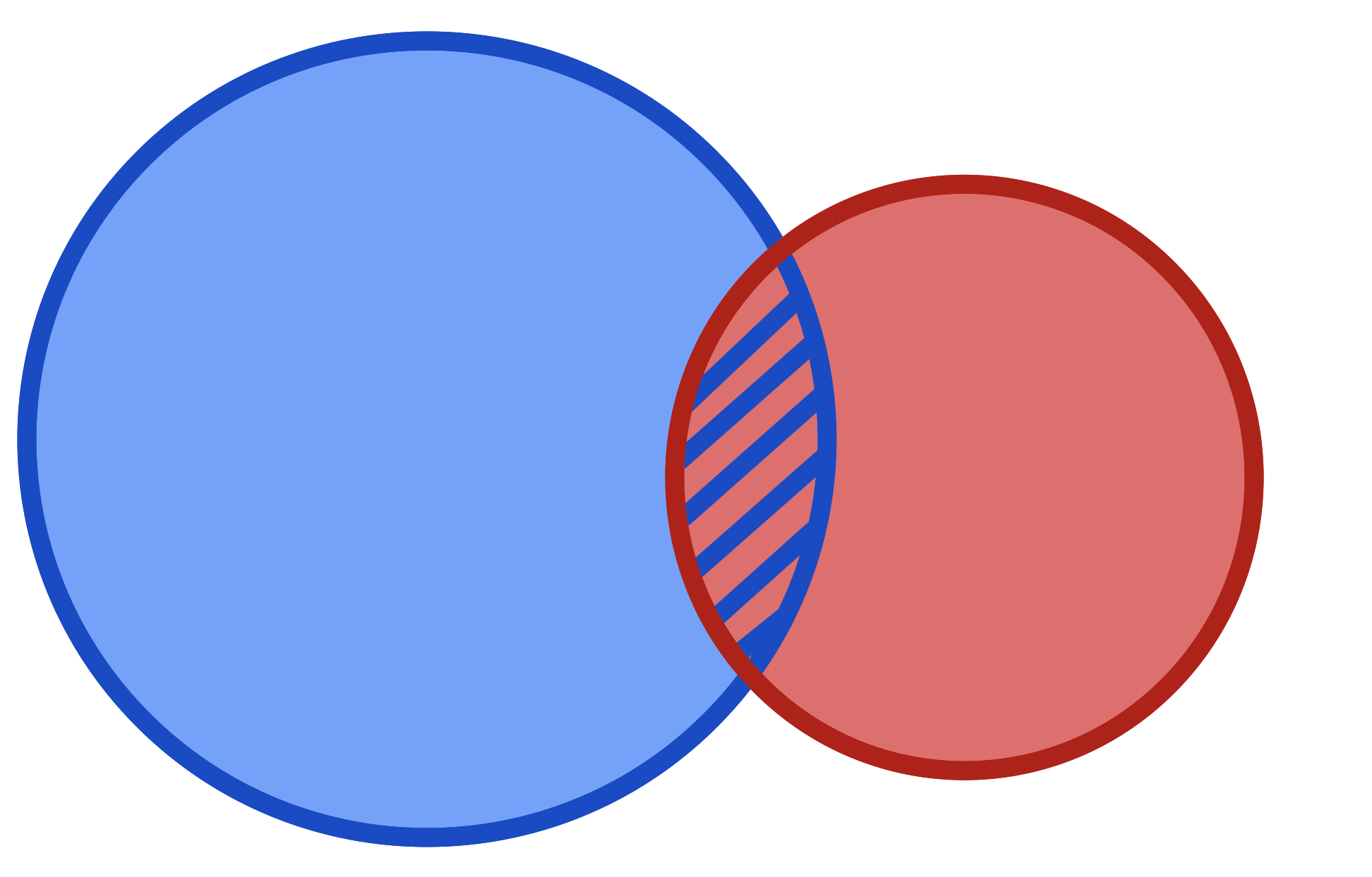
This statement can be visualized using a Venn Diagram:
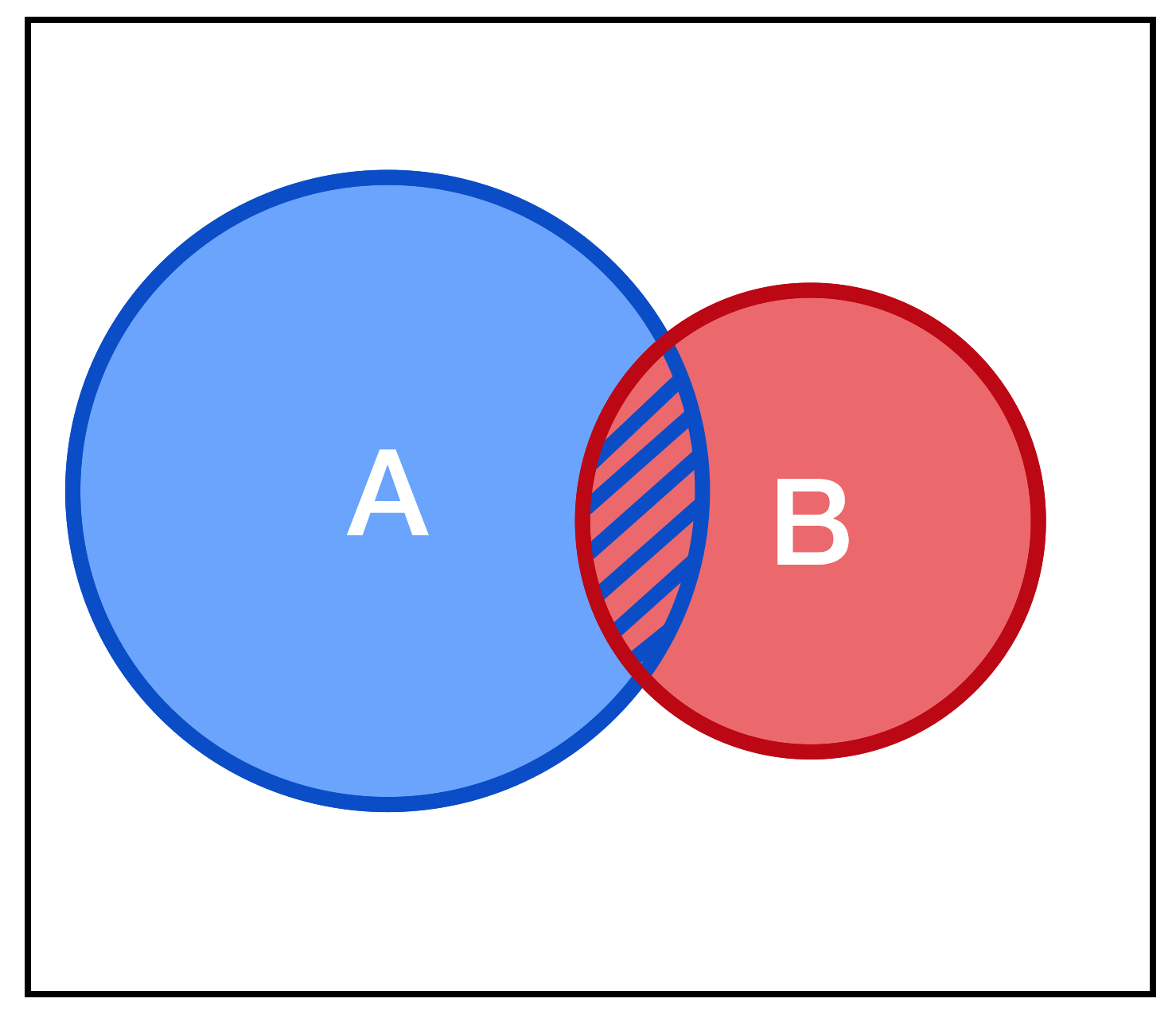
Let's examine what this figure and formula represent. We can think of A and B as two random variables, or two subsets of states a single random variable can take on. Let's start with the latter interpretation, where we have one random variable \(X\) which can take on, among other values, values inside the subset of states represented by A and B, where some states are in both A and B. Area in our two dimensional figure represents probability. The entire outer black rectangle contains the area 1, so all possible combinations of states \(X\) can be in are in this rectangle.
Let's define conditional probability to be: the probability of X being a state inside A given that we know it is in a state inside B. Because we know X is inside B we can immediately ignore everything outside the red 'B' circle in the diagram. That becomes our new universe of possibilities. And now, of that universe, what proportion of it is in A. That's what we're doing by dividing the intersection of A and B by the new 'universe' of B. This is the new probability of A.
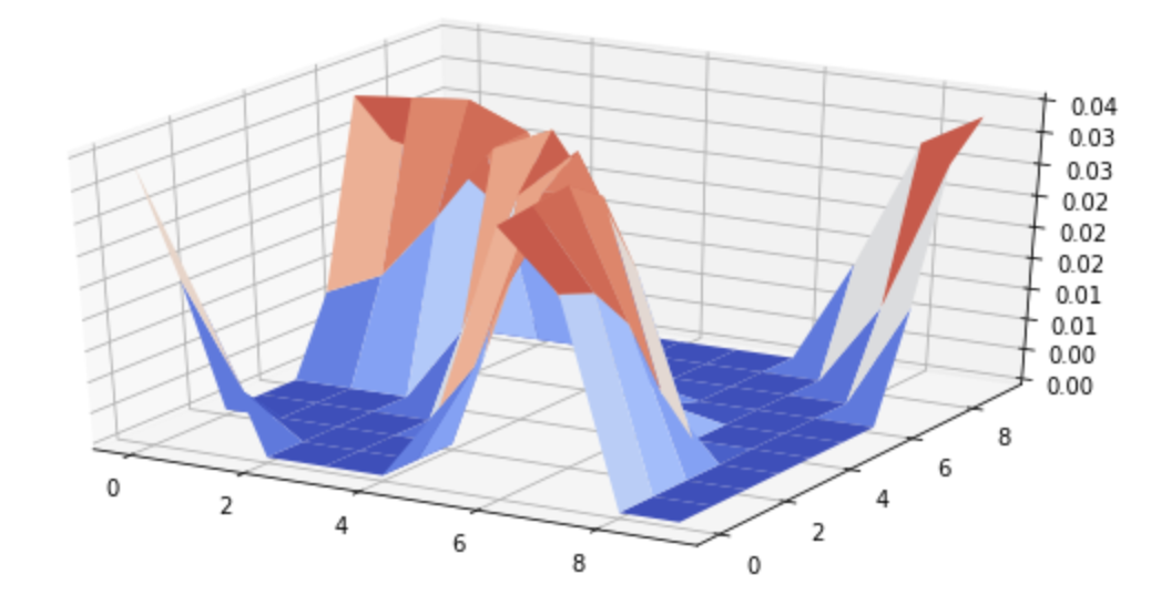
How does this look if A and B represent two variables? Then we are back to our sheet above a plane. A and B are two dimensions, and by conditioning on B we are slicing through B at a particular location b.
Because we are in 3 dimensions (A, B, and \(P(A,B)\)), it's a little harder to visualize than the Venn diagram, but the idea is the same. We're restricting our universe of probabilities to a smaller subset of the original space, and normalizing. The numerator is the original probability along that slice, and the denominator is the total probability mass of our new, shrunken 'universe' where B=b.
To get Bayes' rule from the definition of conditional probability, we can rearrange the terms using algebra.
That's it, that's Bayes' rule! It's the definition of conditional probability, with the numerator expanded using... the definition of conditional probability. Now that we have the rule, how can we interpret it?
Interpretation 1: Hypothesis Testing
Let's replace our As and Bs with ideas. Suppose we are scientists and have several hypotheses about the way the world is. Maybe we have two possible hypotheses:
- $H_1:$ The world is round.
- $H_2:$ The world is flat.
We want to use evidence, or data (d), to determine which hypothesis is true. Bayes' rule then looks like this:
All the parts of Bayes' rule have names.
- $P(H)$ is called the prior distribution. It's the probability distribution among all possible hypotheses before we have any data.
- $P(H|d)$ is called the posterior distribution. Once we've incorporated the data we have a better understanding of which hypothesis is correct.
- $P(d|H)$ is called the likelihood. It answers: assuming we exist in a world in which a particular hypothesis is true, what is the probability of observing this particular data?
- $P(d)$ is the probability of observing the data. This is sometimes very difficult to calculate. In our case with two hypotheses, it's the weighted sum of the likelihoods for the two hypotheses, weighted by the priors of the two hypotheses. In equation form: $$ P(d) = P(d|H_1) P(H_1) + P(d | H_2) P(H_2) $$
Suppose before we observe any evidence, a rational agent would believe that the two hypotheses are equally likely. Then \(P(H_1) = P(H_2) = 0.5\), because the sum of the probabilities for all hypotheses must sum to 1. Now say we perform experiments, make observations, and gather data \(d\). We can calculate the likelihood that we would have observed that data given \(H_1\) is true. This is our likelihood: \(P(d | H_1)\). We can do the same thing for \(H_2\). Now suppose those likelihoods:
$$ P(d|H_1) = 0.01 $$ $$ P(d|H_2) = 0.0001 $$
In general, the probability of observing EXACTLY the sequence of observed data we observed for any hypothesis is going to be small, for the same reason that a particular sequence of heads and tails after 1000 coin tosses is small: there are a lot of possible ways the data could have come out. The important thing for hypothesis testing is how relatively likely they are compared with each other.
Now we have the priors and the likelihoods, we can compute the posterior.
$$ P(H=H_1|d) = \frac{P(H_1)P(d|H_1)}{P(d)} $$ $$ = \frac{P(H_1)P(d|H_1)}{P(H_1)P(d|H_1) + P(H_2)P(d|H_2)} $$ $$ = \frac{0.5 \cdot 0.01}{0.5 \cdot 0.01 + 0.5 \cdot 0.0001} $$ $$ \approx 0.9901 $$
Now that we've incorporated the evidence, a rational agent should believe with over 99% confidence that the world is round.
Model parameters as hypotheses
A special case of hypothesis testing is when you have a mathematical model representing something in the real world, and the different versions of your hypotheses are the different possible states the parameters of the model could take. As an example, let's look at a random variable distributed according to the binomial distribution, parameterized by the (known) number of trials \(N\) and the (unknown) probability of success on any given trial \(p\). For our example let's say we have a clumsy shoelace-tying robot that tries to tie our shoes for us every morning. It's not very good, as it only succeeds 10% of the time. The rest of the time we have to tie our own shoes. Suppose we have just programmed our robot and we don't yet know how good it is at tying our shoes. We are trying to estimate its success rate. Let's call \(\theta\) the parameters we are trying to estimate - in this case only \(p\), the success rate. We observe the robot trying to tie our shoes every day for a week and it fails all but one of those times. Again, let \(d\) be our data. Bayes' rule now looks like:
We haven't tested our robot, so as far as we know, \(\theta\) could be any number between 0 and 1. In this case, we can start with a uniform prior distribution, where all values of \(\theta\) between 0 and 1 are equally likely. Our likelihood is given by the binomial distribution. That is:
Now that we've got our likelihood and prior, we can compute the posterior.
import numpy as np
import matplotlib.pyplot as plt

X = 1
N = 7
delta = .01
p = np.arange(0, 1, delta)
prior = np.ones_like(p)
likelihood = binom.pmf(X, N, p)
p_data = np.sum(prior * likelihood * delta)  # integrate over all possible values of p
posterior = (prior * likelihood) / p_data

fig, (ax1, ax2, ax3) = plt.subplots(3, 1, figsize=(20, 10), sharex=True)
ax1.plot(p, prior)
ax2.plot(p, likelihood)
ax3.plot(p, posterior)
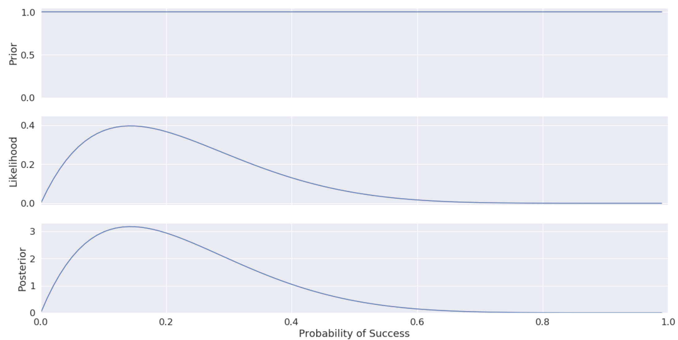
Our posterior distribution is the probability distribution over all possible model parameters. In this case we only have one model parameter, the probability of success. We can see from the graph it peaks around 0.14, although it is still quite spread out. If we observed our robot for more days, the posterior distribution would collapse further around the true probability of success of 0.1.
Interpretation 2: Inverting Causation
To test if C causes E, you perform an experiment where you fix all variables that might influence E, and systematically vary C. If, as you change C, the value of E changes, then you have proven causation. If C doesn't change, then you have proven that C doesn't exert direct causal influence over the E, at least in the particular experimental conditions you controlled.
Causal influence is intuitive to us. Symptoms are caused by diseases. Studying causes students to perform better on tests. Streaming video causes our phone battery to die faster. Wind causes windmills to turn. Much of how we reason intuitively is built on understanding which things cause other things, and which things don't cause other things.
How does Bayes' rule fit into causal inference? Typically, we know the conditional probability of the effect given the cause. This is a natural way of thinking. If I touch the stove, I know the probability I will burn myself. It seems we can store knowledge this way more easily than we can the reverse: suppose I burned myself; what is the probability I touched the stove? If we know the forward, causal probability, we can use Bayes' rule to flip that around and find the backwards, diagnostic probability of the cause given the effect.
Let \(C\) be the cause and \(E\) be an effect. Then Bayes' rule is:
Suppose we have been feeling dizzy and fatigued for the last few weeks and we want to know why. This is a symptom caused by some medical condition or disease. We can figure out the prior probabilities of the different diseases \(P(C_1), P(C_2), ...\) by looking at their rates in the general population or our specific demographic. For each disease we can look at a list of symptoms and a conditional probability table (CPT) to find the probabilities of symptoms given diseases. This is the forward probability, or likelihood. Then, using Bayes' rule in the same manner as we have been, we can compute the posterior probability distribution that we have any given disease. If either the prior or the likelihood for any disease is 0, its posterior will be zero and we can completely rule it out. For instance, if the forward probability \(P(E|C)\) of a hangnail causing dizziness is 0, then we can rule out hangnail as a cause.
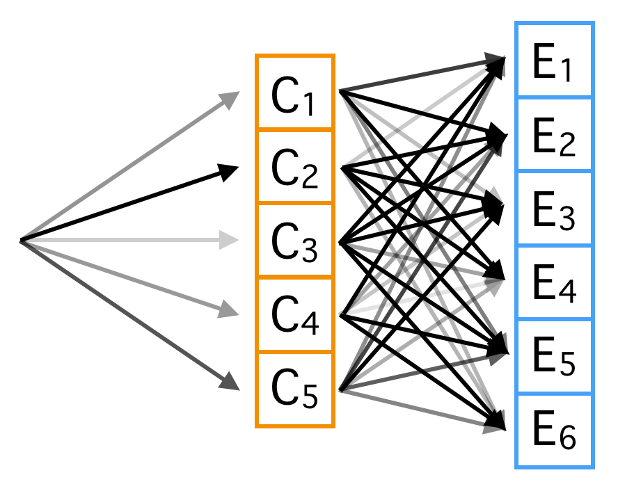
We can interpret this reverse inference in an interesting way. We can think of setting the current state of {disease, symptoms} as moving from left to right in the above diagram. Start at the very left. We imagine there is some causal generative process that first samples from the disease probability distribution, illustrated by arrows of differing thickness. We move to the right to a particular cause. Then we sample symptoms given the disease, we again move to the right, but this time we end up 'activating' multiple symptoms.
The entire forward probability of that happening is just multiplying the weight (darkness) of the first edges we moved along to get to the cause by the weight of the edges we moved along to get to the multiple symptoms. This is the numerator in Bayes' Rule; it is the probability that that particular forward sequence would happen. To get the denominator, we have to calculate those forward probabilities for every possible path in which our observed symptoms are activated. Once we've gotten all the forward probabilities, we just normalize by them to get the distribution over the paths, where each path went through one disease. This gives us the probability of a particular disease.
Conclusion
Bayes' rule is easy to derive, but understanding how it can be applied requires bringing it down from abstract probability theory into the real world of data, hypotheses, models, and causation. Hopefully the ideas in this post helped ground this extremely general and fundamental rule.