Data Generation

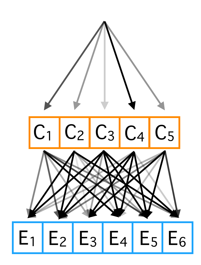
Suppose the data we are analyzing is generated by the procedure shown in the figure above. For each data point, we start at the top. The darkness of the arrows indicates the relative probabilities that a single class will be chosen. There are 5 classes, labeled $C_1$ to $C_5$. We can also think of these classes as 'causes', because each one of them causes the effects at the bottom of the diagram, with probabilities proportional to the darkness of the arrows. The causes are a single random variable that can take 5 states. The effects are 6 binary random variables.

So the entire procedure for data generation is: start at the top, pick a cause according to a probability distribution. Then, the presence or absence of each effect is sampled from the Bernoulli distribution with a probability entirely determined by the cause.

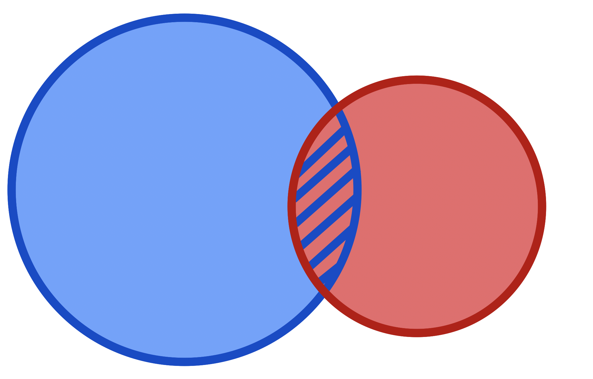
This generative model is a simple example of a Bayesian Network. A Bayesian Network specifies a joint probability distribution with a very useful property: if the value of the parents of a particular variable are fixed, no change in variables anywhere else in the network will influence the value of the variable. In our case, once a particular cause is chosen, if we perform an experiment where we change the value of $E_1$, if will have no influence on the value of $E_2$. Another useful property of Bayesian networks: knowing the value of any variable in the network won't give you any information about any target variable if the values of the parents, children, and children's parents (the variables in Markov blanket) of the target variable are known. In our case this means: conditioning on the value of a cause, knowing $E_1$ won't give you any information about the value of $E_2$. All the effects are conditionally independent when conditioned on the cause. This conditional independence is the property we will exploit to use the naive Bayes classifier.

The central problem: how can we determine which cause was present if we can only observe the effects? To solve this problem we will use the naive Bayes classifier. Before we get into the classifier itself, let's generate data as described above.

Generate Data

import numpy as np
import matplotlib.pyplot as plt
import torch
import pyro
import pyro.distributions as dist

cause_probs = [.1, .05, .4, .25, .2]
def sample_point():
    cause = dist.Categorical(torch.tensor(cause_probs)).sample().item()
    if cause == 0:
        effect_probs = [0, 0, 0, 0, 0, 1]
    elif cause == 1:
        effect_probs = [.2, .2, .2, .2, .2, 0]
    elif cause == 2:
        effect_probs = [.5, .5, 0, 0, 0, 0]
    elif cause == 3:
        effect_probs = [.1, .1, .2, .2, .01, .39]
    elif cause == 4:
        effect_probs = [.05, .05, .3, .3, .2, .1]
    effects = [dist.Bernoulli(e).sample().item() for e in effect_probs]
    return cause, effects

data = [sample_point() for i in range(1000)]
causes = np.array([d[0] for d in data])
effects = np.array([d[1] for d in data])

Naive Bayes Classifier

The naive Bayes classifier uses Bayes' rule and a conditional independence assumption to determine the which class a particular data point belongs to. In our generative framework, this means finding the cause that generated the particular effects we observed. Bayes' rule is given by:

The prior $P(C)$ is easy to to estimate; we can take the distribution of the training data as a good approximate of the true distribution. To calculate the likelihood $P(E|C)$, we can condition on each class, and find the distribution of every possible combination of our 5 effects. These are binary values, so there are $2^6=64$ different probabilities we need to specify to come up with the distribution for each cause. The fact that we need to estimate so many probabilities to come up with the complete distribution is a huge problem, because we probably won't have too many examples of each unique combination of effects to come up with a good estimate. How can we get around this? This is where the conditional independence assumption comes to the rescue. Because the effects don't influence the probability of each other when conditioned on the cause, we can make the following simplification of our likelihood:

Instead of having to estimate 64 different probabilities for each class - one for each unique combination of effect (technically 63, because all probabilities have to sum to 1) - we only have to estimate 6. This is the power of the conditional independence assumption, and of the naive Bayes classifier. Our probability estimates will be much more accurate because have fewer probabilities to estimate, so we have more data per estimate.

Putting it all together, in order to estimate the posterior probability distribution of each cause given the effects, we can compute $P(E=e_i|C=c_j)$ for the 5 $c_j$s and the 6 $e_i$s. Then, when we given a particular data point we want to classify, we multiply these likelihoods together with the class/cause prior probability, and normalize across all classes:

Let's do this in code:

## Get prior
_, counts = np.unique(causes, return_counts=True)
prior = counts / np.sum(counts)

## Get array of likelihoods
likelihoods = []
for j in range(5):
    effects_j  = effects[np.where(causes==j)[0]]
    likelihoods.append(np.mean(effects_j, axis=0))
likelihoods = np.array(likelihoods)

def get_posterior(effects):
    unnormalized_posterior = []
    for j in range(nCauses):
        lj = likelihoods[j]
        l = [lj[i] if effects[i]==1 else 1-lj[i] for i in range(len(effects))]
        unnormalized_posterior.append(np.prod(l) * prior[j])
    posterior = unnormalized_posterior / np.sum(unnormalized_posterior)
    return posterior

cause, effects = sample_point()
posterior = get_posterior(effects)
print(f"Cause: {1 + cause}")
print(f"Effects: {effects}")
print(f"Posterior: {posterior}")
print(f"Predicted Cause: {1 + np.argmax(posterior)}")

Output:

Cause: 3
Effects: [1 1 0 0 0 0]
Posterior: [0 0.014 0.974 0.019 0.001]
Predicted Cause: 3

Here we see that for this data point, the hidden cause was $C_3$. This cause generated effects $e_1,e_2$. Using Bayes' rule with the conditional independence assumption, we calculated our posterior distribution across the 5 possible causes. To make a prediction we took the causes with the highest posterior probability, which in this case was $C_3$. Our classifier made a correct prediction.