Introduction
Most of the time when you want to compare two parameters, like the means of two populations, to see if one is different from the other and by how much, you cannot test every single member of the entire population. You have to take a subset of the population and from that population, estimate what the true parameter would be if you could sample the entire population.
In Bayesian statistics, we treat the parameters we are trying to estimate as random variables that come from a probability distribution. This distribution is governed by Bayes' rule.
The probability that a parameter takes a particular value given the data is proportional to the prior probability that the parameter took that value before the data, times the likelihood of observing the data given that parameter is the correct one.
Once we have the posterior probability distributions of our two parameters, we can ask questions about them, like: Which one is higher? What is the probability that the first is higher than the second? If we have to make a decision that depends on these parameters, and each decision is associated with a cost that depends on the true (unobserved) values of the parameters, what is the decision that minimizes the expected value of the cost?
Bernoulli trials
Very commonly the parameter we are trying to estimate is the probability of success of a Bernoulli trial. Bernoulli trials are things like flipping a coin, a person buying a product on a website, the direction of the price of a stock in a day, or any other event that will have one of two possible outcomes. For our example, we will suppose we are composing a song and we aren't sure whether or not to use one of two synthesizers. We like the sound of both of them equally, but we would like to know if our audience prefers synth A or synth B more. To test this we will make songs with both synths, and when people go to our website, we are going to randomly let them stream either the A or B version. We will record whether or not they finish the song; we will consider a trial a success if they finish the song and a failure otherwise.
For this whole example, we are going to suppose we know the true probabilities of success for both version, if we could sample the entire population of the world. The probability of success for synth A is 40%, and for synth B it is 55%.
Experiment time
We run our experiment for a week, and this is what we come up with:
import pyro
import pyro.distributions as dist
import torch
import numpy as np
import scipy
import scipy.stats
from scipy.stats import binom, beta
import matplotlib
import matplotlib.pyplot as plt
font = {'size'   : 18}
matplotlib.rc('font', **font)
plt.style.use('ggplot')
p_A = 0.4  # True rate for group A
p_B = 0.55 # True rate for group B
true_diff = p_B - p_A

def A_sample():
    A = pyro.sample('A', dist.Bernoulli(p_A))
    return A

def B_sample():
    B = pyro.sample('B', dist.Bernoulli(p_B))
    return B

def run_experiment(N_A, N_B):
    pyro.set_rng_seed(30)
    A_data = np.array([A_sample().item() for _ in range(N_A)], dtype=np.int)
    B_data = np.array([B_sample().item() for _ in range(N_B)], dtype=np.int)
    A_Nsuccess = np.count_nonzero(A_data)
    A_Nfailure = np.count_nonzero(np.logical_not(A_data))
    B_Nsuccess = np.count_nonzero(B_data)
    B_Nfailure = np.count_nonzero(np.logical_not(B_data))
    return A_data, B_data, A_Nsuccess, A_Nfailure, B_Nsuccess, B_Nfailure

N_A = 500
N_B = 200
A_data, B_data, A_Nsuccess, A_Nfailure, B_Nsuccess, B_Nfailure = run_experiment(N_A, N_B)
blue_d = '#0044BD'
blue_l = '#67A2FF'
red_d = '#BE0004'
red_l = '#ED686A'
def plot_AB_hists(A_data, B_data):
    fig, (ax1, ax2) = plt.subplots(1, 2, figsize=(5, 5), sharey=True)
    ax1.hist(A_data, bins=2, range=(0, 1), ec=blue_d, color=blue_l);
    ax2.hist(B_data, bins=2, range=(0, 1), ec=red_d, color=red_l);
    ax1.set_ylabel('Count');
    ax1.set_xticks(ticks=(0, 1));
    ax1.set_xlabel('Synth A')
    ax2.set_xlabel('Synth B')
    ax2.set_xticks(ticks=(0, 1));
    ax1.title.set_text(f'{A_Nsuccess / N_A}')
    ax2.title.set_text(f'{B_Nsuccess / N_B}')

plot_AB_hists(A_data, B_data)
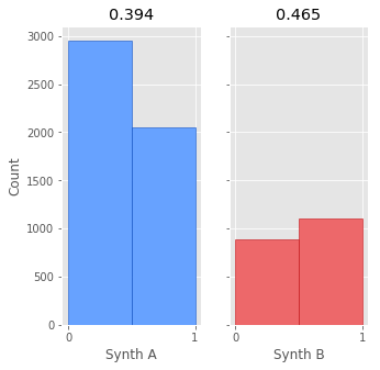
500 people have listened to the song with synth A, 200 to synth B (One of the nice things about Bayesian A/B testing is that you can compare very different sample sizes). The measured proportions of completing the song for A and B are 0.394 and 0.465 respectively. Now that we have our data, how do we we determine which one is better?
Calculating the posterior distributions
If we let \(d\) be the observed data and \(\theta\) stand in for the probability of success in a Bernoulli trial, Bayes' rule is given:
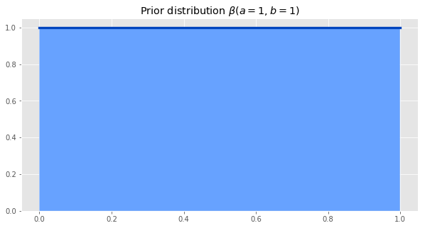
If we have no idea how popular our song will be, and we would be equally surprised if the probability of someone finishing the song was anywhere between 0 and 1, we can choose our prior to be a uniform distribution between 0 and 1. This is the same as a Beta distribution with parameters a=1, b=1.
dx = .001
x = np.arange(0, 1, dx)
prior = beta.pdf(x, 1, 1)
fig, ax = plt.subplots(figsize=(10, 5))
ax.plot(x, prior, color=blue_d, linewidth=3.3)
ax.fill_between(x, prior, np.zeros_like(x), facecolor=blue_l, interpolate=True)
ax.set_title(r'Prior distribution $ \beta(a=1, b=1) $')
ax.set_ylim(bottom=0);
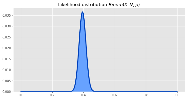
The other part of the formula we need to calculate is the likelihood of particular parameter values generating the data we observed. The likelihood is given by the binomial distribution.
likelihood = binom.pmf(A_Nsuccess, N_A, x)
fig, ax = plt.subplots(figsize=(10, 5))
ax.plot(x, likelihood, color=blue_d, linewidth=3.3)
ax.fill_between(x, likelihood, np.zeros_like(x), facecolor=blue_l, interpolate=True)
ax.set_title(r'Likelihood distribution $ Binom(X, N, p) $')
ax.set_ylim(bottom=0);
Multiplying the likelihood and the prior distributions, and normalizing, gives us the posterior. This posterior is the same as the beta distribution with parameters a = number of successes + 1, b = number of failures + 1, so we will use that going forward.
unnormalized_posterior = likelihood * prior
posterior = unnormalized_posterior / np.sum(dx * unnormalized_posterior)
# posterior = beta.pdf(x, A_Nsuccess, A_Nfailure)  # This is the same posterior as the previous line
fig, ax = plt.subplots(figsize=(10, 5))
ax.plot(x, posterior, color=blue_d, linewidth=3.3)
ax.fill_between(x, posterior, np.zeros_like(x), facecolor=blue_l, interpolate=True)
ax.set_title(r'Posterior distribution $ \beta(a=successes, b=failures) $')
ax.set_ylim(bottom=0);

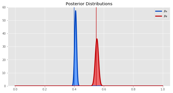
Plotting our posterior distributions for both synths - \(p_A\) and \(p_B\) - together gives us this.
def plot_two_betas(a1, b1, a2, b2):
    fig, ax = plt.subplots(figsize=(10, 5))
    x = np.arange(0, 1, .001)
    pdf_A = scipy.stats.beta.pdf(x, a1, b1)
    pdf_B = scipy.stats.beta.pdf(x, a2, b2)
    ax.plot(x, pdf_A, color=blue_d, label='$p_A$', linewidth=3.3)
    ax.plot(x, pdf_B, color=red_d, label='$p_B$', linewidth=3.3)
    ax.fill_between(x, pdf_A, pdf_B, where=pdf_B <= pdf_A, facecolor=blue_l, interpolate=True)
    ax.fill_between(x, pdf_A, pdf_B, where=pdf_A <= pdf_B, facecolor=red_l, interpolate=True)
    overlap = np.minimum(pdf_A, pdf_B)
    zero = np.zeros_like(overlap)
    ax.fill_between(x, overlap, zero, facecolor='#FF9400', interpolate=True)
    plt.title("Posterior Distributions")
    ax.legend()
    ax.set_ylim(bottom=0);
    ax.axvline(p_A, color=blue_d);
    ax.axvline(p_B, color=red_d);

plot_two_betas(A_Nsuccess, A_Nfailure, B_Nsuccess, B_Nfailure)
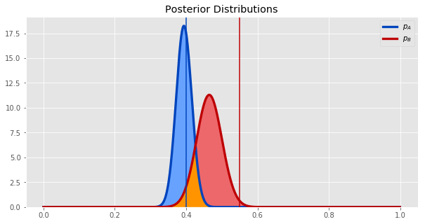
The vertical lines show the true values of the parameters, and the curves show the posterior distribution of the parameters.
It does seem from the plot that synth B is probably better. Let's quantify how much better it is by getting the probability distribution of the difference between \(p_A\) and \(p_B\). We can estimate this by sampling many times from each posterior distribution, taking the difference, and plotting a histogram of the samples of this new random variable.
def B_minus_A():
    A = pyro.sample('A', dist.Beta(A_Nsuccess, A_Nfailure))
    B = pyro.sample('B', dist.Beta(B_Nsuccess, B_Nfailure))
    return B.item() - A.item()
samples_B_minus_A = np.array([B_minus_A() for i in np.arange(10000)])
fig, ax = plt.subplots(figsize=(10, 3))
plt.hist(samples_B_minus_A, bins=200, range=(-1, 1), color='#FF9400');
plt.title("Posterior Distribution of $p_B - p_A$")
ax.axvline(true_diff, color='black');
plt.ylabel('Count');
plt.xlabel('Value');
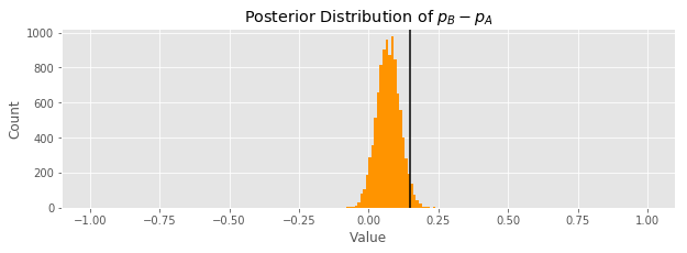
The black line shows the true \(p_B - p_A\). It doesn't fall in the center of our distribution estimating its value, but it is not too far off. Only a tiny sliver of the distribution is below the 0 mark, suggesting that the people enjoy synth B more.
Making Decisions
It does look like B is better than A, but what if we are wrong!? We can still choose between A and B. Here is a twist: in order to use B we have to pay someone else a fixed fee. This means there is a cost to B we have to take into account before making our decision. There is also a cost of picking the wrong synth if the actual population prefers the other one.
Let's formalize this. Suppose the true \(p_A\) = 0.40, and the true \(p_B\) = 0.55. If we had perfect information, the cost of picking B is 0, since B is the better choice. However, we don't have perfect information, so we might choose A. There is a nonzero cost of picking A, but what is it?
Let's make an assumption that our cost is proportional to the difference between the values. Formally:
def cost_A(x):
    k = 50
    return np.maximum(0, k * x)

fig, ax = plt.subplots(figsize=(10, 3))
x = np.arange(-1, 1, .01)
plt.plot(x, cost_A(x), color='#0044BD');
ax.set_ylim(bottom=0);
plt.title('Cost of chosing state A')
plt.ylabel('Cost');
plt.xlabel('$p_B$ - $p_A$');
ax.axvline(true_diff, color='black');
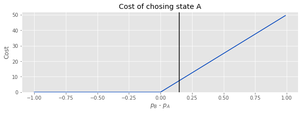
Again, the black line shows the true difference between the parameters.
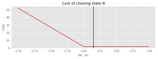
The cost for picking B will be similar, but we will add the cost we have to pay to license synth B (\(s\)) between the states.
def cost_B(x):
    k = 50
    s = 2
    return np.maximum(0, -k * x) + s

fig, ax = plt.subplots(figsize=(10, 3))
x = np.arange(-1, 1, .01)
plt.plot(x, cost_B(x), color='#BE0004');
ax.set_ylim(bottom=0);
plt.title('Cost of chosing state B')
plt.ylabel('Cost');
plt.xlabel('$p_B$ - $p_A$');
ax.axvline(true_diff, color='black');
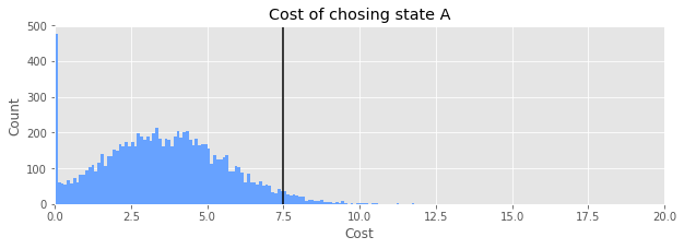
Now we will use the results of sampling our posterior distribution of the difference between \(p_A\) and \(p_B\) to get the distribution of costs for making the different choices.
fig, ax = plt.subplots(figsize=(10, 3))
plt.hist(cost_A(samples_B_minus_A), bins=np.arange(0, 20, .1), color='#67A2FF');
plt.ylabel('Count');
plt.xlabel('Cost');
plt.title('Cost of chosing state A');
print(f"Expected value of loss: {np.mean(cost_A(samples_B_minus_A)):.2f}")
ax.set_xlim(0, 20)
ax.axvline(cost_A(true_diff), color='black');
Expected value of loss: 3.59
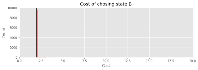
fig, ax = plt.subplots(figsize=(10, 3))
plt.hist(cost_B(samples_B_minus_A), bins=np.arange(0, 20, .1), color='#ED686A');
plt.ylabel('Count');
plt.xlabel('Cost');
plt.title('Cost of chosing state B');
print(f"Expected value of loss: {np.mean(cost_B(samples_B_minus_A)):.2f}")
ax.set_xlim(0, 20);
ax.axvline(cost_B(true_diff), color='black');
Expected value of loss: 2.03
def plot_cost_decrease(samples_B_minus_A):
cost_decrease = cost_A(samples_B_minus_A) - cost_B(samples_B_minus_A)
fig, ax = plt.subplots(figsize=(10, 3))
plt.hist(cost_decrease[cost_decrease >= 0], bins=100, range=(0, 10), color='#ED686A');
plt.hist(cost_decrease[cost_decrease < 0], bins=100, range=(-10, 0), color='#67A2FF');
plt.ylabel('Count');
plt.xlabel('Cost');
plt.title(f'Cost decrease by choosing B. E[X] = {np.mean(cost_decrease):.2f}');
ax.axvline(cost_A(true_diff) - cost_B(true_diff), color='black');
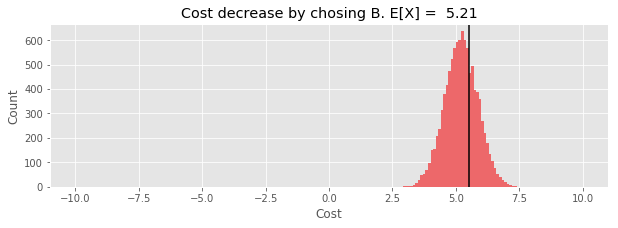
plot_cost_decrease(samples_B_minus_A)
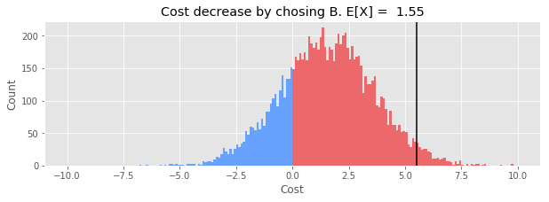
The expected value of the decrease is positive, so we are probably better off making the switch to B.
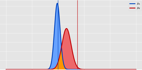
Extending our experiment
If we run our experiment for longer, we can be more sure of which decision is best.
N_A = 5000
N_B = 2000
A_data, B_data, A_Nsuccess, A_Nfailure, B_Nsuccess, B_Nfailure = run_experiment(N_A, N_B)
samples_B_minus_A = np.array([B_minus_A() for i in np.arange(10000)])
plot_two_betas(A_Nsuccess, A_Nfailure, B_Nsuccess, B_Nfailure)
plot_cost_decrease(samples_B_minus_A)